A new map of strain across the western US using GPS data

There is always a focus on the data captured by geodetic instruments during an earthquake, but these instruments are just as busy in the time between earthquakes. GPS/GNSS stations also record the gradual strain that accumulates along a fault until it slips again. A new study presents a fresh analysis of that strain in the western United States.

Where two tectonic plates meet, or where tectonic motion changes across a region, Earth’s crust experiences strain—deformation under stress. When a fault slips during an earthquake, it releases this built-up stress as seismic energy that shakes the ground. By monitoring strain over an area, we can estimate the potential for strong earthquakes and identify the portions of faults at the greatest risk in the near future.

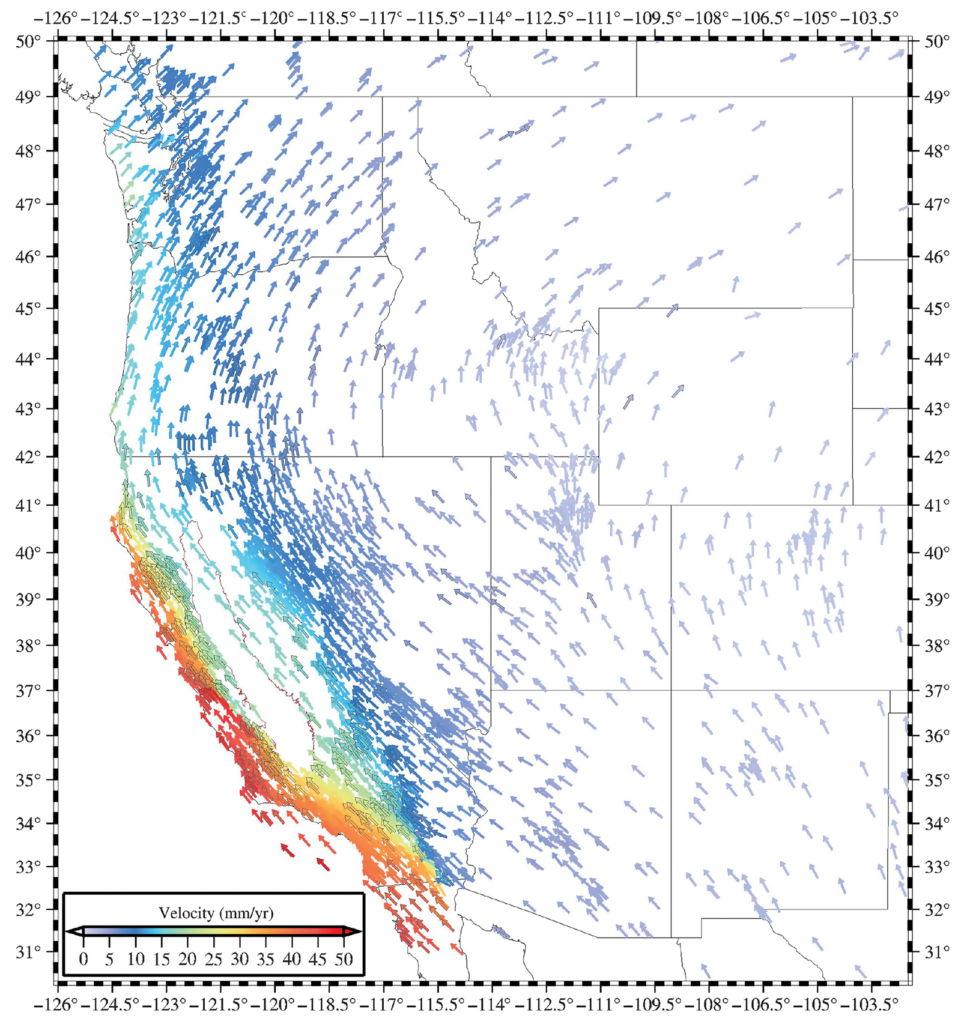
Because a network of geodetic GPS stations measures bedrock velocities in many different locations, it’s possible to map the strain around faults. But this calculation is a little trickier than it sounds. For example, stations near faults will move rapidly during an earthquake—representing the release of strain rather than the accumulation we’re interested in. That means that earthquake-related releases must be removed from the long-term data in order to estimate average strain rates.

Another way to assess strain is to focus on tallying up that release, instead. This can be done by studying the faults themselves, including historical and paleoseismic evidence, to estimate their long-term slip rate. This approach, too, has advantages and disadvantages. It allows the analysis to reach back longer than the GPS network has existed, for example, but we do not have complete data covering every single fault. With perfect data, however, the strain accumulation measured by GPS would exactly equal the strain release measured on faults.

A new study in Seismological Research Letters by Corné Kreemer and Zachary Young at the University of Nevada, Reno combines both approaches. They use data from the Network of the Americas and other archived GPS measurements, as well as a database of fault slip estimates. In addition to maps based on each, they blend the two for a “combined” solution. In each, the rate of strain is represented by color, with red areas accumulating strain the fastest and presenting the greatest earthquake hazard.

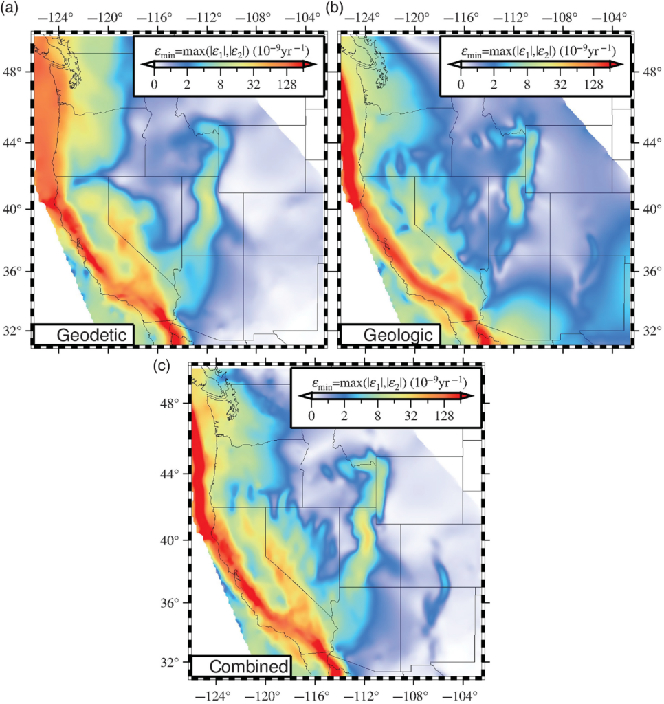
The combined map concentrates more of the strain closer to specific faults, like the San Andreas Fault system in California. It also highlights Basin and Range extension in Nevada, in part because of a correction applied to the Pacific Northwest. Along the Cascadia subduction zone, the subducting oceanic plate is pushing on the continental plate, squeezing it eastward. This is measurable in eastern Oregon and Washington, even though the actual fault zone is offshore, and has the effect of obscuring some of the extension in next door in northern Nevada.

The study then compares the strain map to observed earthquakes. Specifically, the researchers looked at the correlation between strain rate and the number of earthquakes (leaving out aftershocks) in each location. It’s expected that, all else being equal, the number of earthquakes should increase linearly with increasing strain rate.

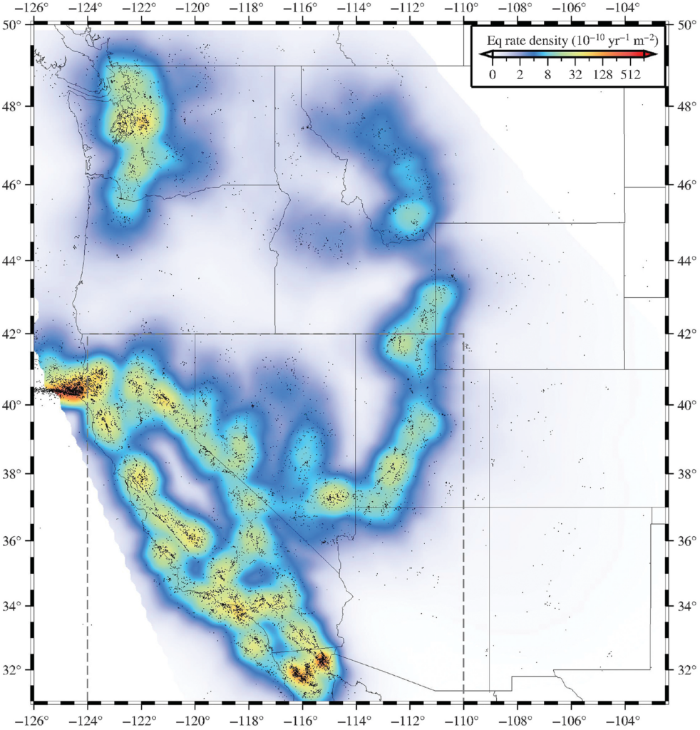
For the southern portion of the region, the team found an interesting departure from this tidy relationship. There was a kink in the linear relationship, with the number of earthquakes increasing more slowly above a given strain rate. There are a number of possible explanations for this difference between low-strain and high-strain areas like the San Andreas. For example, the Cascadia subduction zone—which was purposefully excluded—releases strain in comparatively few but very large earthquakes. There could potentially be a similar difference in behavior between the high-strain San Andreas Fault system and lower-strain faults in the region. Or it may be that multiple differences in fault characteristics are involved.

The goal of all this, of course, is to better understand local earthquake hazards. By employing new methods for analyzing those hazards, we can attempt to fill in any unknown blind spots in that understanding—and eliminate surprises.