Choose the correct type of data source, which is indicated by the Data Source Type entry box. Data Source Type "I'm Feeling Lucky" is appropriate for NetCDF grids; this choice also works for some other data sources the IDV can recognize. For others you must select another type, such as "netCDF Point data files." or Text Point Data Files for "point data" - data values at scattered locations on on inside the Earth.

Browse to the data item you want to connect to the IDV, click on it, then click Add Source.

For more see Choosing Data Sources (some meteorology data sources described there are not available in the UNAVCO IDV).

Selecting parameters ("fields") to display, and creating displays

See The Field Selector

You choose (click on) a Field name in the "Field Selector" tabbed panel in the Dashboard, then click on a display type under Displays, and then click on the "Create Display" button. The IDV offers only display types suitable for the character of the data.

A "Plan view" is a horizontal cross section. "Cross sections" are all vertical cross sections.

Managing displays of point data has a separate section in this how-to.
For examples of all the kinds of geophysical data displays in the UNAVCO IDV, see Geoscience Data, Displays, and online Data Sources.

Zooming, Panning and Rotating

The IDV is a true 3D display system. IDV controls for zooming panning and rotating are more complex than is common for other computer displays, since it is a true 3D system. There are two or more ways to pan, zoom, and rotate. Once you learn them, it is very powerful. Until you learn them it can be a little confusing or surprizing.

See Zooming, Panning and Rotating

Google Earth-like controls can be used. Choose main menu choice Edit->Preferences, Navigation tab, and click on Google Earth. See also Edit Preferences. You can change how the IDV interprets mouse and keyboard events for navigating in 3D space. For each combination of mouse button and control/shift keys you can select an action. There are a number of navigation functions (e.g., rotate) that can be triggered by a key press. The Keyboard preference tab allows you to define the key and any modifier (i.e., control, shift).

Other controls on point of view change the projection, change the vertical scale, change the point of view of a 3D display with View->Viewpoint->Viewpoint dialog, and turn on auto-rotation in the globe display.

Reset Point of View

If you get the display in some confusing point of view, hit Control-r to reset the view. The view now is the full "projection," and in the strictly overhead view.

Viewpoint Controls

The left border of the main window has viewpoint and "zoom/pan" contols which are very useful. See Viewpoint Toolbar and Zoom/Pan Toolbar. That web page also describes Apple Mac One Button Mouse controls.

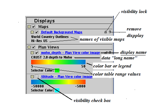
Display Legends and Controls

The Display Legends area appears on the right side of the main data display window when the IDV starts up. As you add data displays and choose maps, legends for each item appear here. You get controls for the displays with the legends. For more about using the legends, see Display Legends.

Display controls are key to using the IDV. They are a collection of controls gathered in one window, to control one display of one data source in one main map view or globe view window. Each display may have different controls, depending on its data source. To get full value from the IDV you need to have a good understanding of display controls.

Click on one display name to pop up its associated display control in the Dashboard window.

For a full discussion of display controls, see Display controls.

Here are a few basic tips.

Click the visibility check box to hide a display from one data set; when you do this the display is not removed and it is easily restored by clicking the visibility box again.

Click the remove display button to permanately remove the display.

Do a right click on the color bar to see the color table controls menu. You can choose a different color table, and change the range of data values associating values with colors.

The display name is made of two parts : before the hyphen the variable name, a single word, from the netCDF data file. The second part is from the IDV, the display type name such as "Plan view color image" or "Plan view as contours."

The data's "long name" comes from the "long_name" attribute for the data in its netCDF file. The figure shows a display long name of "CRUST 2.0 depth to moho." If there is no long name in the netCDF data file it may not be clear which display control or display goes with which data set. Be sure to use the long_name in your netCDF files.

Click the visibility lock icon to ensure a display is always visible when you cycle visibility. This is a very useful way to compare data sets.

The Projection

A key concept in using the IDV is the "projection." An IDV projection is a geographic area to display, with an associated transform from the round earth to a flat map view (the actual map projection). In most cases it is best to use a projection area which is close to the area covered by your data set, especially for displays of data with depth. The IDV includes standard projections; use menu choice Projections -> Predefined. See also the Unidata IDV help page Changing Projections.

To make a projection for your area,

You may need to adjust the vertical scale (see below) to get good results from your data in a projection.

The IDV may reset the projection everytime you add a new data set. To turn this off, check off the box

Projections -> Autoset Projection (old term Reset projection with new data).

Make Your Own New Map Projection

You can make a new map projection of almost any kind.

See Projection Manager.

Choose main menu item Projections -> New/Edit

In the Projection Manager that pops up, click on the box "New."

In the Define Projection window that pops up, enter a name.

Select a Type such as Transverse Mercator.

Enter the appropriate control values.

Click Preview. A sketch of the new projection appears in the map window.

You can drag the corners of the outline in the map window.

Click Save.

The new name is now in the list of projections in the Projection Manager window,
and in your main menu Projections -> Predefined list.

Map Controls

Maps are provided in the IDV. Use the main menu choice Displays -> Maps -> Add System Map and click on a suitable map. You can add your own map with a map "shape file." Each Projection used in the IDV is initially provided with a "background map" (which you can turn off if you like).

Maps appear in the list of Displays on the right side of the main IDV window. Click on a map name such as "Map display" or "Background maps" to open the display control window for the map display.

In a display control window for a map, the "Maps" tab panel allows you to toggle on and off the display with the check box, change color of line (click on the color box), and change line thickness and style.

In a display control window for a map, the "Display" tab panel allows you to turn on or off latitude and longitude line (two check boxes), set their spacing in degrees, line style, and change their color. You can slide the map from the bottom to the top of the wireframe box (which may not be visible; see wireframe box and vertical scale control information).

Maps in the list of Displays on the right side of the main IDV window can be toggled off and on with the check box, or permanately removed by clicking on the trash can icon on the right edge.

The Wireframe Box.

The IDV display may include a 3D wireframe box that provides a sense of 3D orientation, and position points in the vertical dimension. You turn on or off the wireframe box with the menu choice View -> Show -> Show Wireframe box. The vertical scale, next, sets the top and bottom depths (or altitudes) of the wire frame box. Depths below the Earth's surface are negative, increasing downwards.

If the display outside the wireframe box is not wanted, you can it off with View -> Show -> Clip at wireframe box.

To show a scale along the vertical edge of the wireframe box, use View -> Show -> Show Display Scales.

On start up the normal wireframe box is 40% as high as it is wide. To change the vertical aspect ratio of the wireframe box (other than 40%) use the View->Properties menu. Go to the aspect ratio tab.

Vertical Scale

Vertical scale or vertical exaggeration in 3D plots is under user control. The vertical scale sets the top and bottom depths of the wire frame box. Depths below the Earth's surface are negative, increasing downwards. A side view of any 3d display (see Viewpoint toolbar), with the "not converging to infinity" selection in the same toolbar, allows you to read out the depth of any point with the mouse cursor. If displaying point data, be sure to click on the Declutter padlock (see below).

Vertical scale works best with a projection that just includes the area covered by your data. To get the tool to change the vertical scale, use the bottomn button in the " Viewpoint toolbar," or in the IDV use the menu choice View->Viewpoint->Vertical Scale. You enter max min and units for depth values. For data below the earth surface the depth values are negative and the vertical range should have a max of say 0 and a min of perhaps -100. Be sure the units are what you want.

To show a scale along the vertical edge of the wireframe box, use View -> Show -> Show Display Scales.

To make a 1:1 vertical exaggeration (same distance scaling in depth as horizontally):

• set your display to overhead view (as use ctrl-r keys)
  
• turn on the wireframe box with View -> Show -> Show wireframe box
  
• get the range and bearing measurer, with Displays->Special->Range and Bearing
  
• move the ends of the range and bearing line in the display by mouse drags until it spans the middle of the wireframe box; note the width in the readout, such as "Distance 671.8 km."
  
• get the vertical scale tool with the botton button in the " Viewpoint toolbar," or in the IDV use the menu choice View->Viewpoint->Vertical Scale.
  
• Make the distance interval between Min and Max to be 0.40 times the distance across the wireframe box. The wireframe box height is 40.0% of the width [always?].
  
• This is only approximate in most map projections; the smaller the area covered the more exact it is.

To change the vertical aspect ratio of the wireframe box (other than 40%) use the View->Properties menu. Go to the aspect ratio tab.

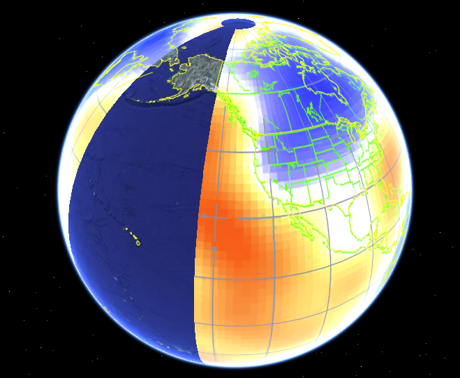
The Globe Display

The IDV can make a 3D globe display. To open a globe display, choose File -> New -> Display Windows -> Globe Display -> One Pane. Then use the Field Selector window as usual to make a display. Some displays work well in the globe, including point data plots such as earthquake locations, plan Views, and 3D isosurfaces.

To see solid earth data in the globe display for the entire Earth to the center, some settings must be correct.

Visibility Cycling for Data Comparison

A good way to compare two displays is to quickly cycle visibility between them. Use the F1 key to flip between two or more displays
The F1 key cycles visibility through all non-locked displays, showing one at a time.
The F2 turns on all non-locked displays.
The F3 turns off all non-locked displays.
(On a Mac laptop, you may need to press the "Fn" key along with the particular function key.)
The visibility lock icon is used to block the effects of the visibility toggling. When locked, the visibility of a display is not affected by the toggling.

Display Background Color

You can select the color of the display background and lines in drawings such as maps with the main window menu choice View -> Colors. Click on a preset combination such as "Black on white," or select your own colors with "Set Colors."

Saving IDV displays as images and movies

You can save a display as a static image (jpeg, gif, or png format file). You can also save movies of displays with animation, or with moving points of view, or with any other change in the display such as adding more data plots.

To save an image of your display use menu choice View->Capture->Image and enter the file name. To make the largest possible image, first select main menu choice View -> Full Screen. To shrink back from full screen, click the same menu choice again.

You can capture movies of time animation of data, or sequences of rotation, zooming; or a any sequence of displays you can make. See Image and Movie Capture for complete instructions. You can save moveis as Quicktime format or as an animated GIF file that will display on any web page. Animated gifs are generally smaller than Quicktime files.

IDV Bundle Files

IDV "bundle files" let you save a quick "snapshot" of the IDV, including data sources, maps, and data displays. Bundles are very useful, when you see all they can do. You may end up using IDV bundles all the time.

Bundles are information files that specify the state of the IDV. They include information about what data sources are used to make a display, and which parameters from the data sources are displayed, and how they are displayed. Map projections and areas, point of view, and color table choices are saved. Bundles are small enough to attach to email; they do not (usually) have "real data" in them.

The purpose of bundles is for you to save a particular IDV setup and display. A bundle can be used for your own reference at a later time. Others using can use your bundles to see IDV displays you make. Bundles facilitate data exchange and comparisons.

To make a new bundle file select the menu choice File -> Save As. A pop-up window lets you set a file location and name. The IDV adds the file extension .xidv to the filename. An IDV bundel file is also called an 'xidv' file. The format is XML.

To use a bundle file, use, in the main display window, File -> Open. Find and open a bunlde file. The IDV will find the data sources specified in it, connect to all the data sources, read in the data needed to make displays, and create the displays exactly as you created them. You will be asked if you want to retain or remove any existing setup in the IDV before opening the bundle file.

Here are different and important uses for bundle:
- to save work in progress to resume later
- to archive a data display that shows something of interest to you.
- to save one or more special IDV configurations you use with certain kinds of data
- to share with colleagues, locally or by email
- to post online for many others to see your IDV displays
- to encapsulate IDV setup for a classroom or lab exercise, homework, etc.
- to encapsulate completed lab exercises or homework using the IDV, to send to the instructor.
- to preserve demos of IDV use

Special Bundles

You can save the unique "default bundle" with menu choice "File -> Default Bundle -> Save." This bundle controls what the IDV does when it starts up. You can save a common map and projection and data choices this way, so you do not have to recreate common settings by hand. If you have data in a some source you regularly check, the IDV can display it the same way each time you start the IDV with no menu choices.

You can save "favorites" which are just names for bundle files. To save one do the menu choice "File -> Save as Favorite" to see a popup box that allows you to catalog and name favorites. To display a favorite, do the menu choice "Displays -> Favorite Bundles." You can also open (File -> Open) any bundle file from your system, from online, or anywhere, to use that bundle to determine what you see in the IDV.

Saving IDV displays as KML and KMZ files for Google Earth

You can save an IDV display as an image in a KML or KMZ file for use Google Earth. In Google Earth this is a single item, layer or image; you cannot interact with the data as you can in the IDV.

In the IDV to make a kml file, you do menu choice View->Capture->Image-> Files of Type Google Earth, and include the .kml file extension in the name.

To make a proper KML file, the IDV display must be in two states: a pure lat-long map projection (which is all GE can use) and a pure overhead map view. Set that up before you do the KML file capture. One way to do this is to choose the IDV menu choice Projections->Use displayed area.

To make the largest possible image with highest resolution, select the menu choice View -> Full Screen. To shrink back from full screen, use view-reset full screen.

Sample Google Earth views showing seismic tomography displays made in the IDV:
   
Tomography values by color at 350 km depth; 3D isosurfaces from tomography.

Unfortunately the Google Earth views of such interior data can be misleading; only surface data should be used this way in most cases.

Text Notes

The IDV has a provision for you to record text notes, either stand-alone or associated with a display. These notes can be saved in Bundles, so you use can use these to describe displays for others, annotate classroom exercises, have students return homeworki with answers attached as bundle files, etc. Bundles are files of information that allow the IDV to recreate a previous state of data and displays.

To create a stand-alone text note choose from the main menu Displays->Special->Text note. A window opens where you compose the note, in the Dasboard window. If you want to float the note in a liitle window so it is more visible, click on the little up arrow icon below the text note entry box.

A text note you save with a bundle will appear on the screen when the IDV loads the bundle. You can also attach a note to any or all individual parameter displays through the properties window: Edit->Propertiesi; click on "Show Text Note." The text area will be opened in the bottom of the window in which you can compose your note.

Subsetting 3D Grids (reduce memory demand for displays)

In a gridded data source, you can subset the data points to just the region you want to display. In the Dashboard's Data sources panel, do a right-button click on the data source name; then select the Properties menu choice. In that window choose Spatial subset tab. Selecting, for example for a grid, "Every other point" for X Stride and Y Stride will reduce the number of data points to plot by a factor of 4. Point data can be subset by a region box, or with bounds in longitude and latitude.

Seeing NetCDF file Metadata

NetCDF files used by the IDV have metadata describing what is in the file. You can see the metadata. In the Dashboard window's Field Selector window, Data sources panel (left side), do a right-button click on the data source name; then select the Properties menu choice. Click on "Metadata."

Point Data Plots

Many geophysical data are "point data," data values at random locations on or inside the earth, such as earthquakes, GPS vector observations, and strain observations. The UNAVCO IDV has display symbols for such data (which use special variable names in data files).

To connect point data sources to the IDV, in the Data Source Chooser, use "Data Source Type" of "NetCDF point data for geophysics." Or, if you are using csv ascii files, no special type selection is needed; the filename extension .csv is the indicator of file type to the IDV (see IDV_for_GEON_csv.html ).

When you make a display of point data, the Point Data display control window pops up:

The Declutter check box turns on "decluttering" which is automatic reduction in how many points are plotted. When Declutter is checked, the Plot density slider provides some control over how many points appear.

The IDV changes which points to plot if you rotate or change the viewpoint. This can be prevented by clicking on the tiny "padlock" icon to the right of the Declutter check box.

Layout model (formerly Station model) is IDV terminology for plot symbols for point data. The figure shows the list opened, showing all the plot symbol types for the UNAVCO IDV (not the Unidata IDV). The location of point data can be shown with the two location symbols. The 3D cross is the simplest symbol making less demands on making many points. As the UNAVCO IDV evolves this list will change.

The "Scale" entry box lets you enlarge or reduce any symbol to any size. Symbol sizes automatically change when you zoom to roughly stay the same size on screen; Scale lets you alter how big they are on screen.
BUG: After zoom the symbol size changes to a previous size. Just click the "Apply" button next to the Scale entry box again.

The "Only show every" choice is for data with differing time values. "Vertical Position" is for data with depth (altitude). Generally most IDV users do want 3D plots with depth, the default selection.

Working with the Point data Plot Symbols using "Layouts Models"

You can modify the provided UNAVCO IDV point data symbols in some ways, making a new plot symbol.

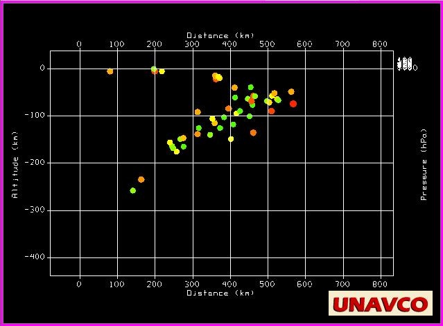
Here is an example, adding color-by-depth to the "Locations-3D cross" symbol. Plot some data that spans say 100 kilometers depth in it, using the Locations - 3D cross symbol.

In the main menu choose Tools->Layout Model Editor (in version 2.1; in older versions do Edit->Resources->Point Data Display Layouts" (or Station Model).

The "Layout Model Editor" window pops up. Choose "Layout Models-> Locations 3D cross." Put the mouse cursor at the exact center of the white display in this window. Right click (mouse button three) to get a menu; choose "Properties." In the Properties window that appears, click the "Color By" tab.

Enter this settings: Color By: Altitude; Depth Range -200 to 0; Unit kilometers; Color table "Basic->Bright 38." You can of course use other depth ranges, units, and color table choice to suit your data.

Click on "Apply" and your main data display will be change to show color with depth. Click "OK" to end the Properties window.

Choose "File - > Save As" to save this "layout model" for future use on your system. Use a name such as "Locations - 3D cross - colored by depth." You can send this new color table to others with an IDV bundle file (see web page here about that).

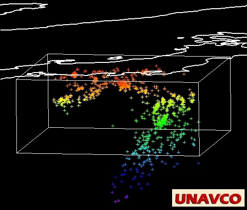
Earthquake locations under Japan (data provided by Francis Wu); click for larger view.

Color a Point Data plot symbol using Layout Models

You may wish to color all of one set of point data symbols one color, and another set with a different color. You can do this if they come from different data files or sources, so each set and display has its own color table.

Use main menu choice  Tools->Layout Model Editor.

Choose Layout Models -> Seismic wave polarization (for example)

Right click, for a popup menu, on the symbol in the white display; choose Properties

Click on the tab named Color By

click on the Color Table: Set box; choose a "solid" color table such as  Solid > Red or Solid  > Blue

TIF Imagery

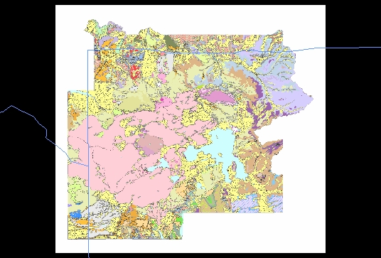
(geology map image provided by Robert L. Christiansen)

To display a navigated TIF image (.tif file)

TIF Imagery Draped over Topography

You can drape a TIF image over 3D topography relief.

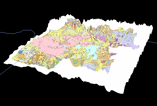
Yellowstone National Park surface geology map drapped over 3D relief topography; oblique view.
(geology map image provided by Robert L. Christiansen)

Follow these steps

JPEG Imagery Mapped with Latitude and Longitudes

You can display a rectangular JPG image which has known limits in latitude and longitude.

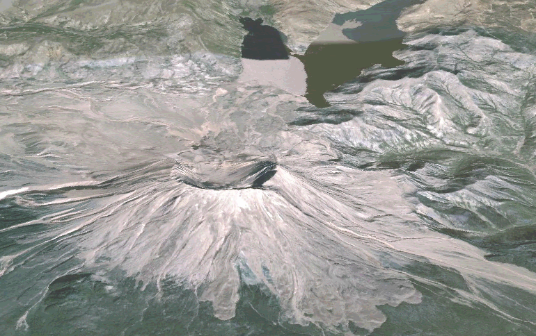
Mt. St. Helens surface photograph, mapped to lat-lon with an .ximg file, and drapped over 3D relief topography; oblique view.

Follow these directions from Unidata:

There is an xml format that allows you to specify the lat/lon bounds of an image. Your xml filename should have a .ximg suffix and look like:

< collection name="Images">
< image
name="Sketch Plan"
url="sketch.jpg"
ullat="39.991856"
ullon="-105.226944"
lrlat="39.989426"
lrlon="-105.222656"/>

< image name="Flood Map"
url="map.jpg"
ullat="39.993625"
ullon="-105.227973"
lrlat="39.98692"
lrlon="-105.22132"/>

< /collection>

Just load in the file through the data chooser. The IDV recognizes the ximg file suffix and creates the right kind of data source. The url can be a file name or a url. It can also be an absolute or relative (to the ximg file) path, as on your local disk.

You have two display types: "3 color image", and "3 color image drapped over topography." For the second you will be asked to indicate the topography data file you have for the same area.

Color Tables

IDV displays of colored images use a "color table" to associate every data value with a color to display each data value. The intent is usually to choose a spectrum of colors that highlights data features. Different data need different color tables; a color table of surface air temperature, from say -20 to 30, would not be of much use for ocean depths of -4000 to 0. The data values limiting the ends of the color table data are called the range.

The IDV comes with many color tables, and a powerful editor tool to modify color tables and make new ones.

Color tables are a very effective way to highlight data of interest, show patterns in data, and generally make displays more understandable and meaningful. If you learn to use color tables you will make displays that highlight important features in your data.

Compare these two vertical cross sections of earth structure made with exactly the same data, but using different color tables. The left image uses the default UNAVCO IDV color table, the right uses a color table tailored to show details in this data set. Click on an image for a larger view.

To select a color table, right-click on the color bar in the Displays legend area on the right side of the main IDV window (there is one color bar for each display that has a color table) to see a drop down menu that lets you:

• select from the many provided color tables, from submenus such as "Basic." Even though some color tables have names associated with a particular data type, you can use any color table for any data type.
• change range of the color table, the data values at the upper and lower ends of the color table. Setting the range is necessary to associate the colors with the data values you want to see.
• see the Color Table Editor with the color table for that display. See The IDV Color Table Editor for how to modify and create color tables.

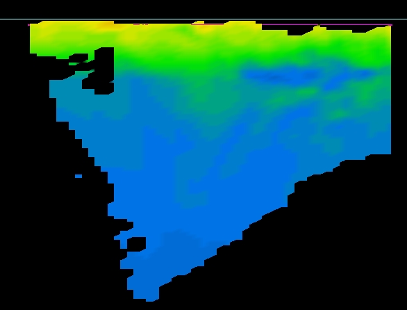
Data provided by Francis Wu, Binghamton University.

Sampling Data Values in the Display

When any data display is colored by value, move the mouse cursor over the color bar in the legend to get the value for each color. This is not precise but sometimes is useful.

With Point data displays on screen, in the "Point Data" control window, click on the tab "Data Readout." Set the display to one of the perpendicular views such as overhead using the Viewpoint toolbar. Click on a point data symbol in the display. The Data readout shows values for that point's data.

For point data, in the Data Selector window one display type is Point Data List. Click that and click Create Display to see a list of all the data in the data set. it does not tell you what point on the display is which one in the list but it can be useful.

There are several "Probes" in the IDV to subset or sample data. See Probes. The "Data Probe" lets you sample values in a 3D field. The "vertical profile" probe shows data along a vertical line through a 3D field, a kind of sounding if you like.

Multiple NetCDF files, one for each time, for time animation

If you have data in multiple NetCDF files, with a time for each one, you can link them in the IDV to allow time animation loops. From Unidata support:

Assuming you are running a fairly recent version of the IDV you can do a multiple select (using Control-Click) of the files in the file chooser. Under the "Data Source Type" select "Aggregated Grid files"

This uses a generated NCML (http://www.unidata.ucar.edu/software/netcdf/ncml/) wrapper and only works if the files differ on time. -Jeff McWhirter

On-screen Color Scale Legend

To add a color scale legend to your display, click on the display control name on the panel on the right side of the main display. The display control pops up. Choose Edit (in the display control, not the outer dashboard border) --> Properties --> Color Scale.
Check the "Visible" box. Click one of the four "Positions" for the scale. Click the "Label Color : Change" box to choose a color for the text values along side the color scale. Click OK or Apply to see the color scale label in the display.

Click for full size

Time Animation with Accumulating Point Symbols

You can show a kind of time animation where more data appears on the screen as time advances, the earlier values not being removed. This is useful, for example, to show aftershock locations filling a fault zone, or lightning strikes locations delineating a thunderstorm.

Load a point data file into the IDV, where each point has its own time value (not all the same times). "Create Display" for a Point Data Plot. Switch off Declutter in the display control window (Layout tab).

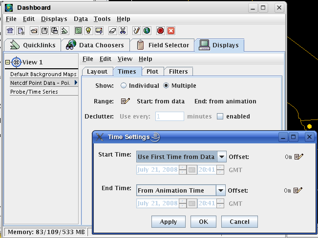
In the display control window, Times tab, check Show : Multiple. Also click on the check item right of "Range" and choose "Start Time: Use First time from data" and "End Time: From Animation Time." See the example above. Click on time animation to see the accumulating plot by time.

Here is a bundle file that shows time accumulating animation for the 200 largest earthquakes in an area including California since 1964. Load the URL for this bundle file in Dashboard window - Data choosers - URLs entry box.

You can use the time animation controls to change the speed of the display. And of course this is a 3D display, showing locations in depth if you change the view from overhead. You can see the parameters for a particular earthquake. Stop the time animation. Click on the Plot tab in the display control. Click on an earthquake in the map display (overhead point of view works best here).

How to increase available memory used by the IDV on a Mac

Here is the way to edit the memory limit on the Mac. The IDV performs much better with 1000 mb or more.

The IDV install on the Mac OS X comes with the maximum memory preset for 512 mb. In order to increase the memory to say 1024 mb, you need to edit the Info.plist file in the IDV application contents. To do this first go into the IDV folder in the Applications folder and holding the Control button on the keyboard and click on "IDV". For a 3-button mouse just right click. This will give the Contents of the file in a new window. Then click on Contents folder. You can edit the Info.plist file by dragging it into a text editor or into a terminal window (type vi first). After the line VMOptions is the memory setting "-Xmx512m". Change this to -Xmx1024m and save the file. You can now launch the IDV by double clicking on the IDV application. You should see 1024 MB as the allocated memory at the bottom of the IDV window.

Alternatively for unix types: in a terminal window type vi /Applications/IDV_2.1/IDV.app/Contents/Info.plist where IDV_2.1 is the version (directory) of your IDV install.

Do not use the maximum amount of memory on your machine as some is needed for the operating system itself. For a system with 2 Gb of physical memory, you can probably allocate 1.5 Gb to the IDV. If you have less than 1 Gb of RAM, you should start the IDV with about 1/2 of the total memory (512 MB). (Unidata)

At present, you really cannot go much beyond 1.5GB, even if you have more memory. The "32 bit limit" is still in the JRE [Java] ....some day (soon?) they'll go beyond this. (Tom Whittaker)

The "Transect View" a vertical cross section for all data types

For any data with a vertical depth character, including point observations such as earthquakes, you can make a special vertical cross section display called a "Transect View" which collapses all the data in a vertical box (of preset width) into a flat display. See online Transect Views, or in the IDV menu, Help -> Main Window -> Transect View. You can control the width of the box that bins the data to show in the transect view display.

First create a Transect display. In the main IDV window, choose File -> New -> Display Window -> Transect Display -> One Pane. The new display opens in it's own window.

In your main (map) display move to an area with overhead map view of the general area where you want the transect. In the new window, make menu choice Transects -> Edit. This brings up the Transect Drawing Control. A color transect line labeled B and E appears on the map display.

In the Transect Drawing Control, Controls tab panel, click on the crossed line symbol. Now you can use a mouse drag in the map display to drag either end of the transect line.

In the Transects Display, under menu item Transects, click on the transect you want to use, which are labeled by end position in latitude, longitude.

Now in the Transects Display, under menu item View, choose Properites, Transect tab. Set the width of the box you want. Any data points outside the box in the map view will not appear in the transect display.

To see vertical scale, in the Transects Display, under menu item View, choose Properites, Vertical scale tab, and enter your vertical scale and units. Some fiddling may be needed to get the display and vertical exaggeration you want. Typical values for data inside the earth are, for example, Min value -600.0, Max value, -100.0 km, Units km.

Finally you can add the data. Make a display like normal in the main window, and the same data will appear in the Transect Display. You can move the position of the transect line, vertical scale, width, and plot symbols (Layout manager).

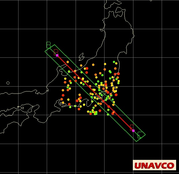
A map display of earthquakes in Japan colored by depth, showing the transect line (red) and box width (green); click for full size

the Transect View from its own window; click for full size

How to put a vertical image in the IDV

This is only available in IDV verison 2.1 which is due before the end of December 2006.

In an ximg file (see Mapping an image into the IDV display) you can, optionally, specify all four points of the image in 3D space with ullat/ullon/ulalt, urlat/urlon/uralt, lllat/llon/llalt, lrlat/lrlon/lralt The IDV fills in some default values if they are not fully specified. e.g.: < image ullat="30" ullon="-100" urlat="30" urlon="-90" ulalt="5000" llalt="0" name="vertical" url="test.jpg"/> In the above we define the altitude (in meters for now) of the upper left of the image to be 5000. The lower left is 0. Since there isn't any alt defined for the upper right or lower right they default to 5000 and 0 respectively. Likewise, since the lower right lat/lon and lower left lat/lon are not defined they default to the lat lon of the upper right and upper left points.

Check out this sample ximg file (for the display below) Geology cross section ximg file.

Geology cross-section of Maryland, a jpg image in the IDV (oblique view):
Click for full size

Using other IDV tools a 3D relief topo map has been included. It can be semi transparent, and moved to any level vertically as well.

A Jython Method to subset a large image, with user input

To learn about data computations with Jython (Python) inside the IDV, see IDV Formulas and IDV Jython Methods.

You can subsample an image with the following Jython library method (called by an IDV "Formula"; see Help about Formula):

def subsample(image, nskip):
  from ucar.unidata.data.grid import GridUtil
  return GridUtil.subset(image, int(nskip))

subsample(image, numpts[isuser=true])

which prompts you for the number of points. Contributed by Don Murray.

See the main how-to page for how to display ("navigate") an image, i.e., set lat/long bounds.