The IDV is a powerful way to visualize and analyse tomography data.
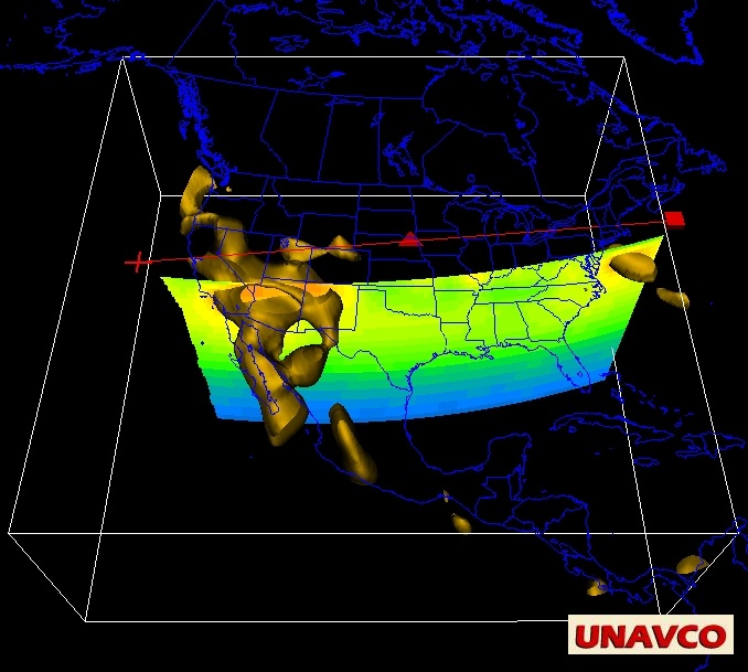
DNA10-S tomography model, oblique 3D view with isosurface of -3.0 percent Vs deviation, and a plan view at 125 km. Actual IDV displays are fully interactive, with rotation, zoom, color settings, and vertical scaling. Click for full size image.
Contents:
Seismic Tomography Model Data from IRIS
Seismic Tomography Model Data from UNAVCO
Sample Displays
Comparing Western US Tomography models
Use the IDV to Compare Different Model Results
Seismic Tomography Model Data from IRIS
IRIS
provides recent seismic tomography model data files in NetCDF format which can be used in the IDV
with no format changes.
Adding the IRIS tomograhy files to the IDV
See the IRIS EMC Earth Models page and select the model of interest. On its page use the link for "the netCDF binary for the model."
Save the model file. In the IDV use the Dashboard window's Data Choosers tab to browse Files and "Add Source."
Use the Dashboard window's Field Selector tab to choose the parameter to display, and the Displays tab to choose the type of display to make.
Then click Create Display.
Another way to use this data is to have the IDV directly read the IRIS EMS data file. On the IRIS EMS page for a model, do "copy link location" (right mouse click) on the same link to the IRIS NetCDF file. Then in the IDV use the Dashboard window's Data Choosers tab, URLs menu option (left frame), enter the link (URL) to the IRIS data file, and click "Add Source." The IDV can now read from this remote data file when it makes a display.
See sample IDV displays made with this data.
Seismic Tomography Model Data from UNAVCO
UNAVCO provides recent seismic tomography model data files in NetCDF format which can be used in the IDV
with no format changes.
Seismic Tomography and the IDV
The IDV is for exploration of complex Earth science data in 3D. With the IDV you can discover and examine features difficult to see
in other ways.
With seismic tomography models the IDV can:
The IDV has true 3D displays and fully interactive controls. Once your data is in the IDV, you can make many kinds of
displays to highlight and bring out details of seismic tomography models. You can use any vertical scale, most any map
projection and area, or a globe display. You can change your point of view to any angle,
and zoom and rotate. You can use the color scale controls to highlight significant features.
You can display other geophysical data in your tomography displays, to compare with the tomographic results.
You can difference and display two tomographic models. You can include seismic raypaths to see coverage densities.
Isosurfaces can be colored by other parameters,
such as values of uncertainty or resolution, so you can judge the quality of the results.
The IDV can do computations with any data source it reads, including differences between
3D tomography models. Different 3D grids need not have the same resolution or grid Earth mapping for the IDV to use them in computations.
The IDV handles grid mappings and unit conversions.
Astronomers use "blink comparators" to show differences between two star fields. With the IDV you can do blink comparisons of
tomography models to quickly see differences.
You can save displays as image files, as KML files for Google Earth
(only as overhead map views of the surface, of course, since that is what Google Earth does),
and as movies (gif or Quicktime) of changes of view.
The IDV uses NetCDF format files. To put data in NetCDF, see
D
Using the NetCDF Data Format for Seismic Tomography.
UNAVCO converts standard models to NetCDF on occasion, to make them available online.
Sample IDV Displays of Seismic Tomography Models
Model name
map extent (resolution)
depth extent;
levels parameter;
unit;
range NetCDF file
data source or report online
Citation
MITP, January 2010
lat 10-70; long 150 W to 50 W (0.20 deg)
25-1000 km (40 levels)
Vp offset from AK135;
percent; -2.2 to 2.9 MITP_USA_2010JAN.nc
Electronic supplement; Model Update 2010
Burdick, S., Li, C., Martynov, V., Cox, T., Eakins, J., Astiz, L, Vernon, F.L., Pavlis, G.L., Van der Hilst, R.D., Upper mantle heterogeneity beneath North America from travel time tomography with global and USArray transportable array data, Seismo. Res. Let., vol. 79 no. 3, 384-392, May/June 2008
UO_wUS_6_10 June 2010
lat 26.65-50.15; long 126.3 W to 98.8 W
(0.25 deg) 60-990 km (20 levels)
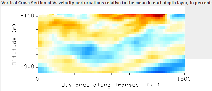
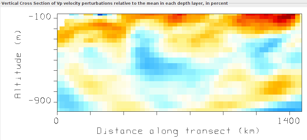
Vp and Vs perturbations relative to the mean in each depth layer
in percent (-4.634 to 5.49; Vs perturbations) UO_wUS_6_10_dVp.nc
UO_wUS_6_10_dVs.nc
Schmandt, B., Humphreys, E., Complex subduction and small-scale convection revealed by body-wave tomography of the western United States upper mantle, Earth Planet. Sci. Lett. (2010), doi:10.1016/j.epsl.2010.06.047.
SEMum
global
surface - 2891 km deep (21 levels)
Voigt average VP, VS, and anisotropic parameters ξ = VSH2/VSV2 φ = VPV2/VPH2
http://seismo.berkeley.edu/~lekic/SEMum.html
Lekic, V. and B. Romanowicz, 2011, Inferring upper-mantle structure by full waveform tomography with the spectral element method. Geophys. J. Int. 185(2), 799-831.
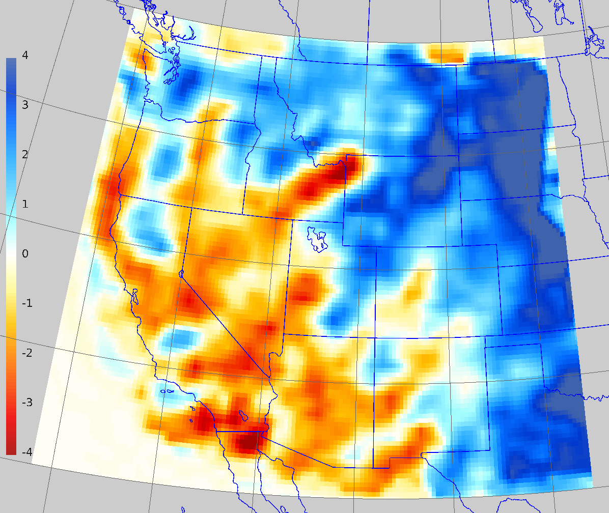
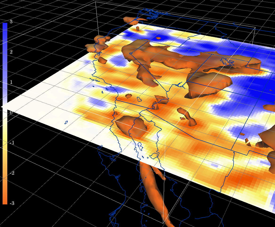
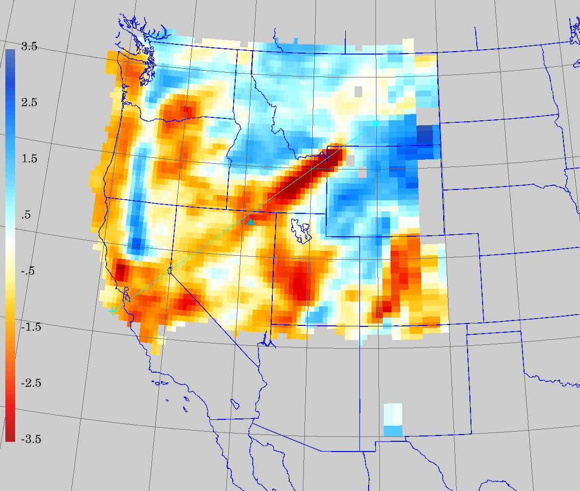
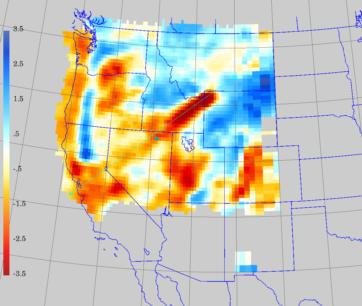
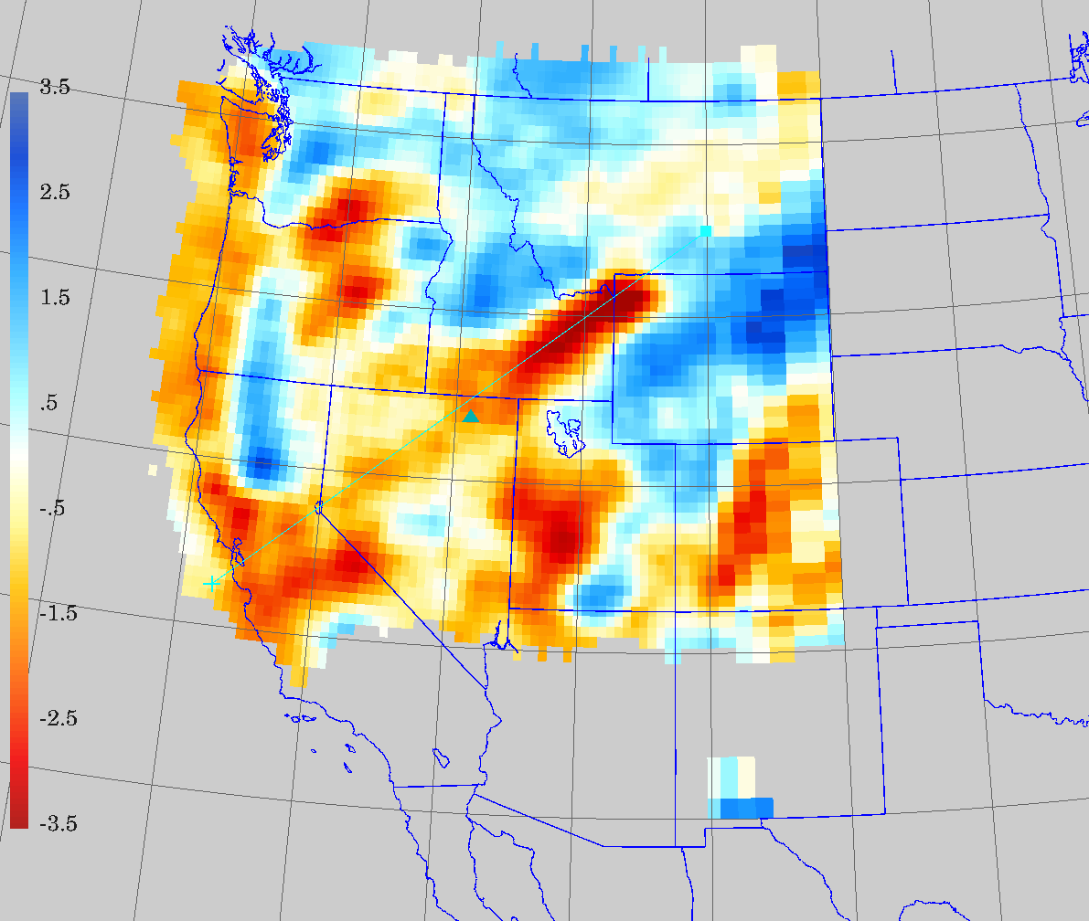
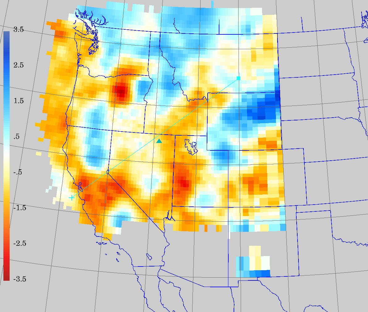
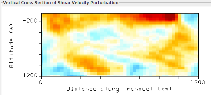
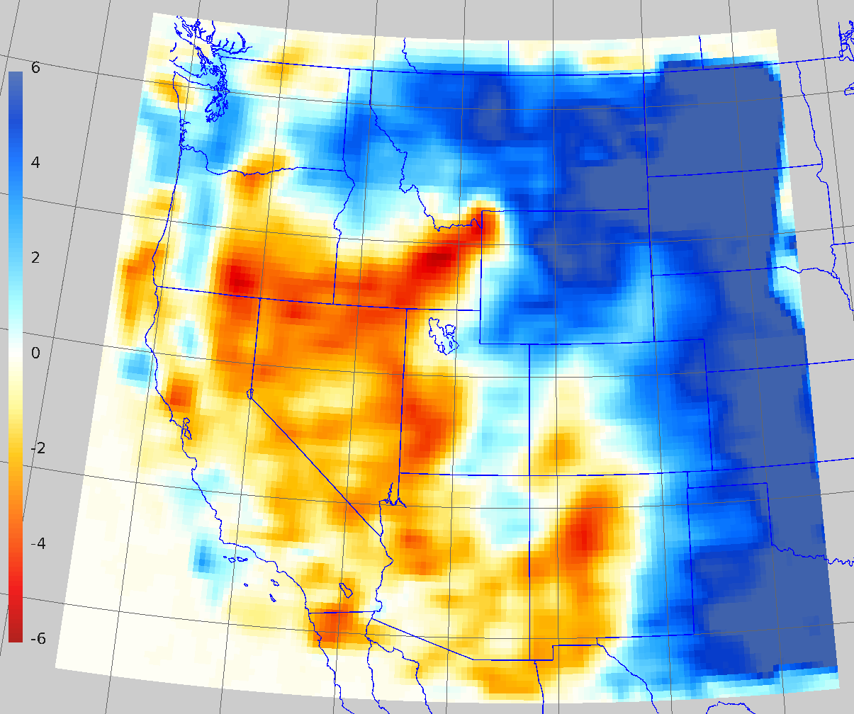
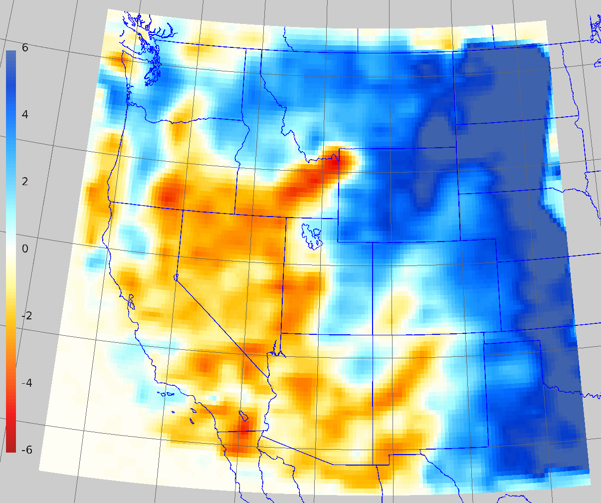
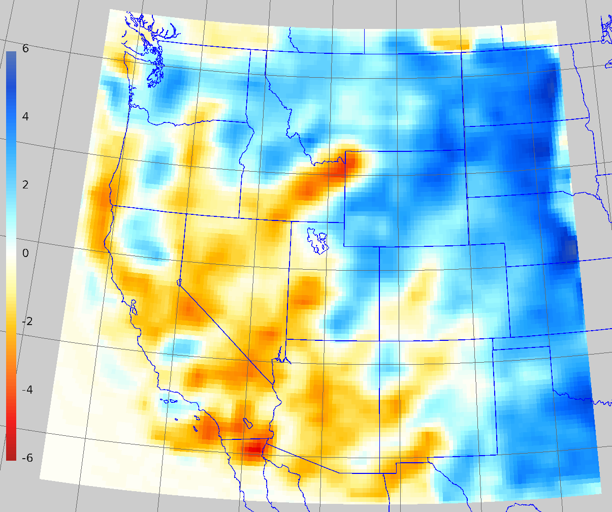
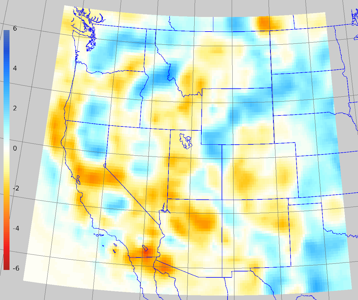
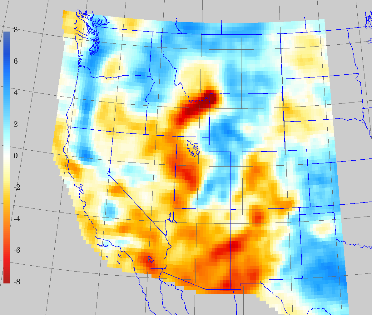
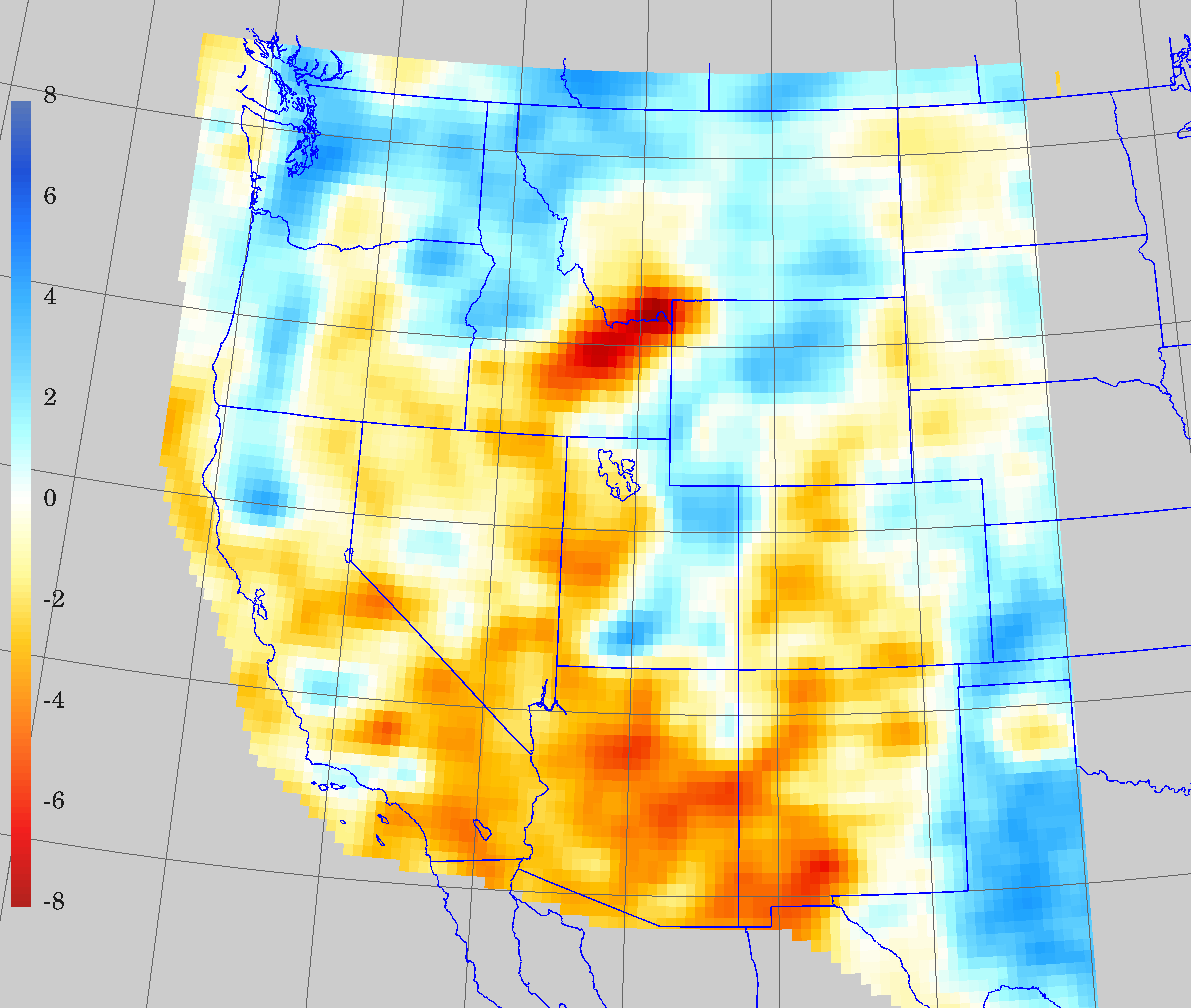
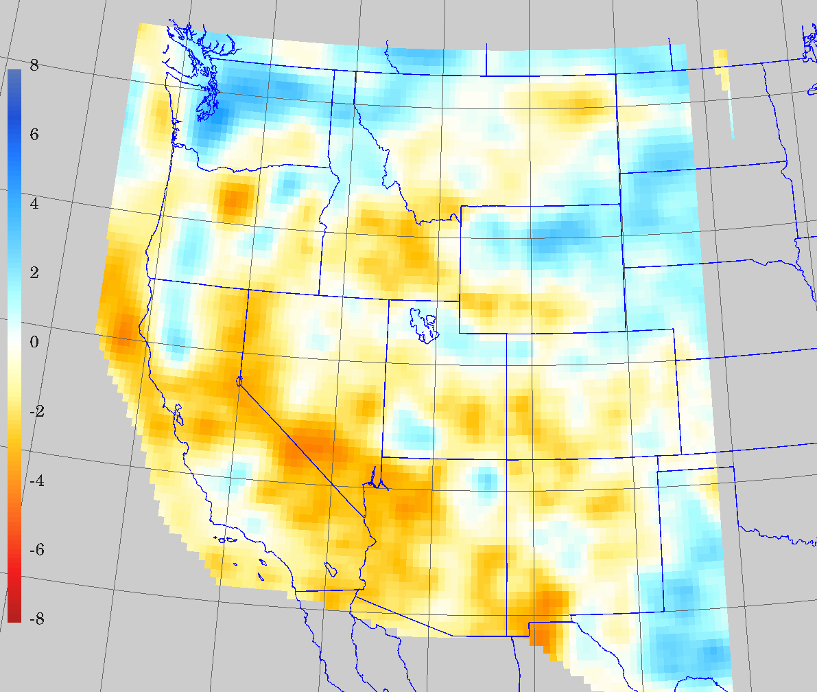
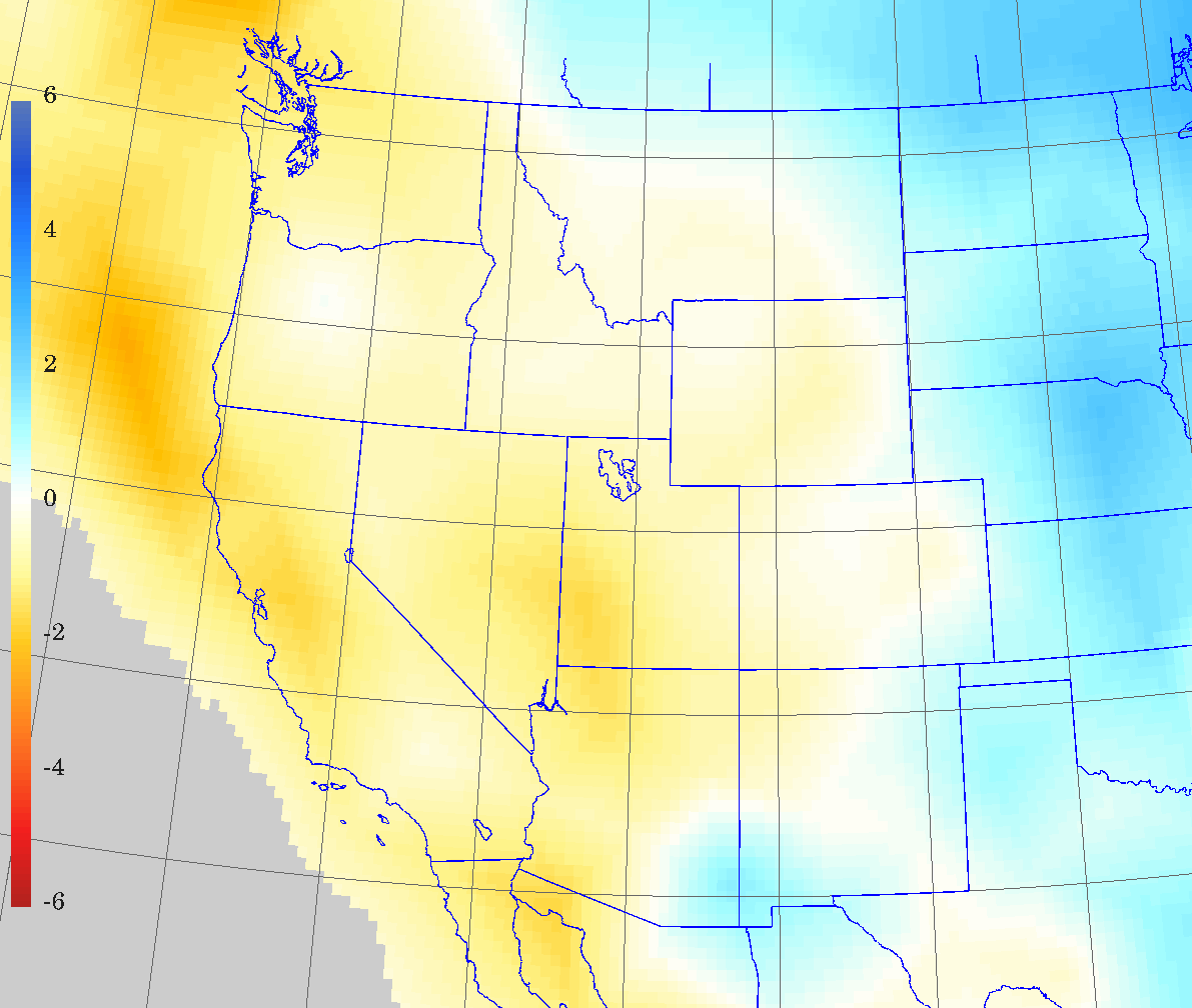
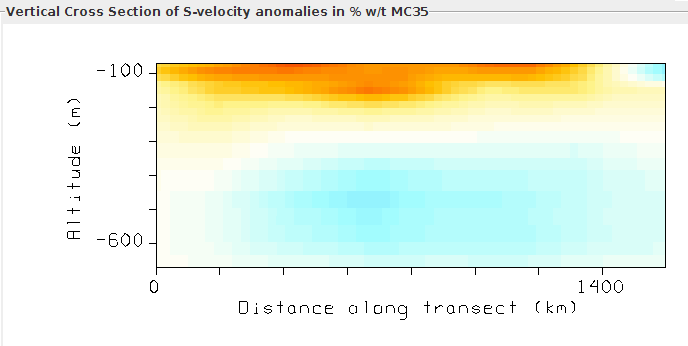
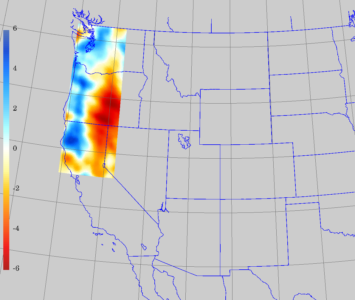
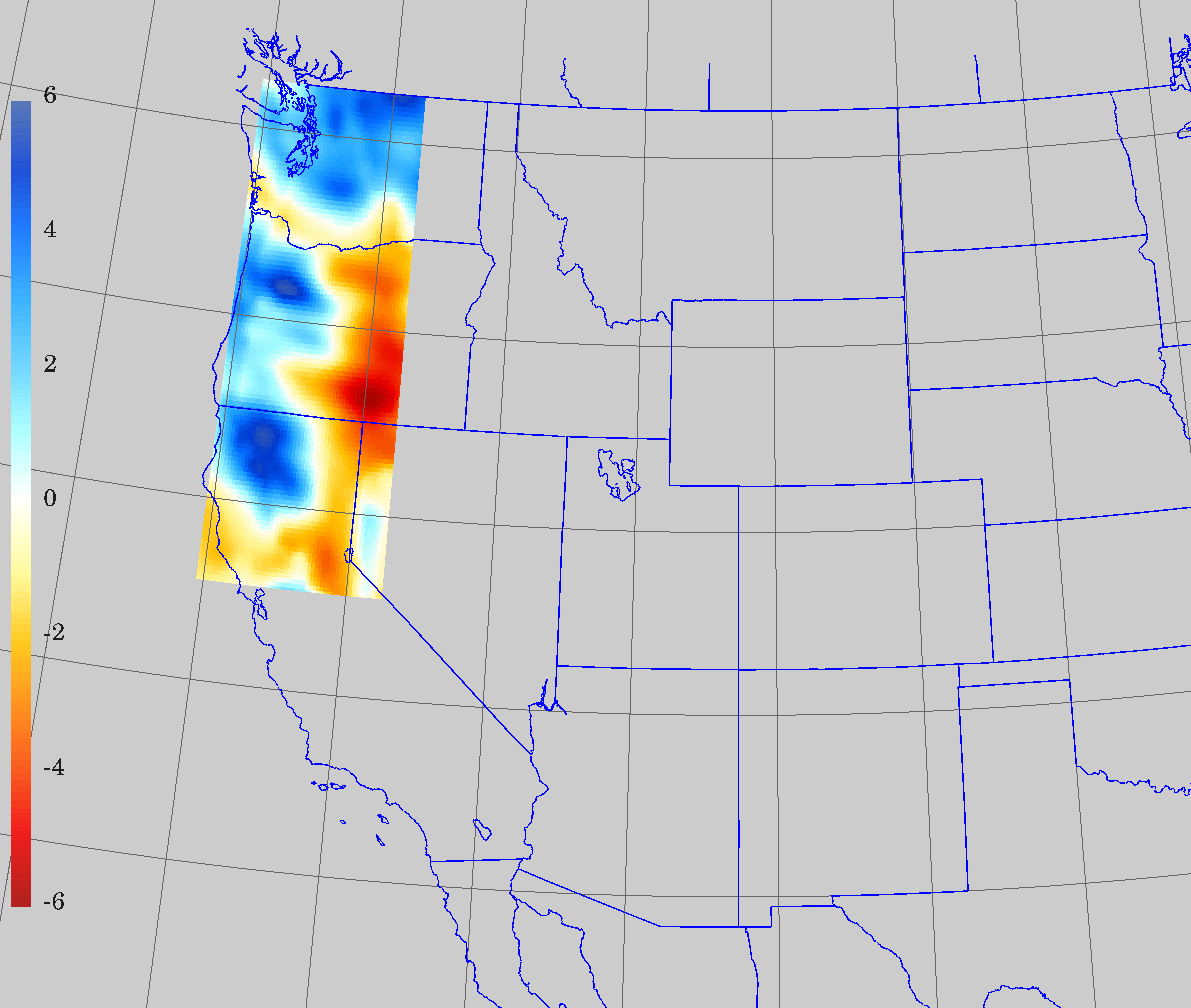
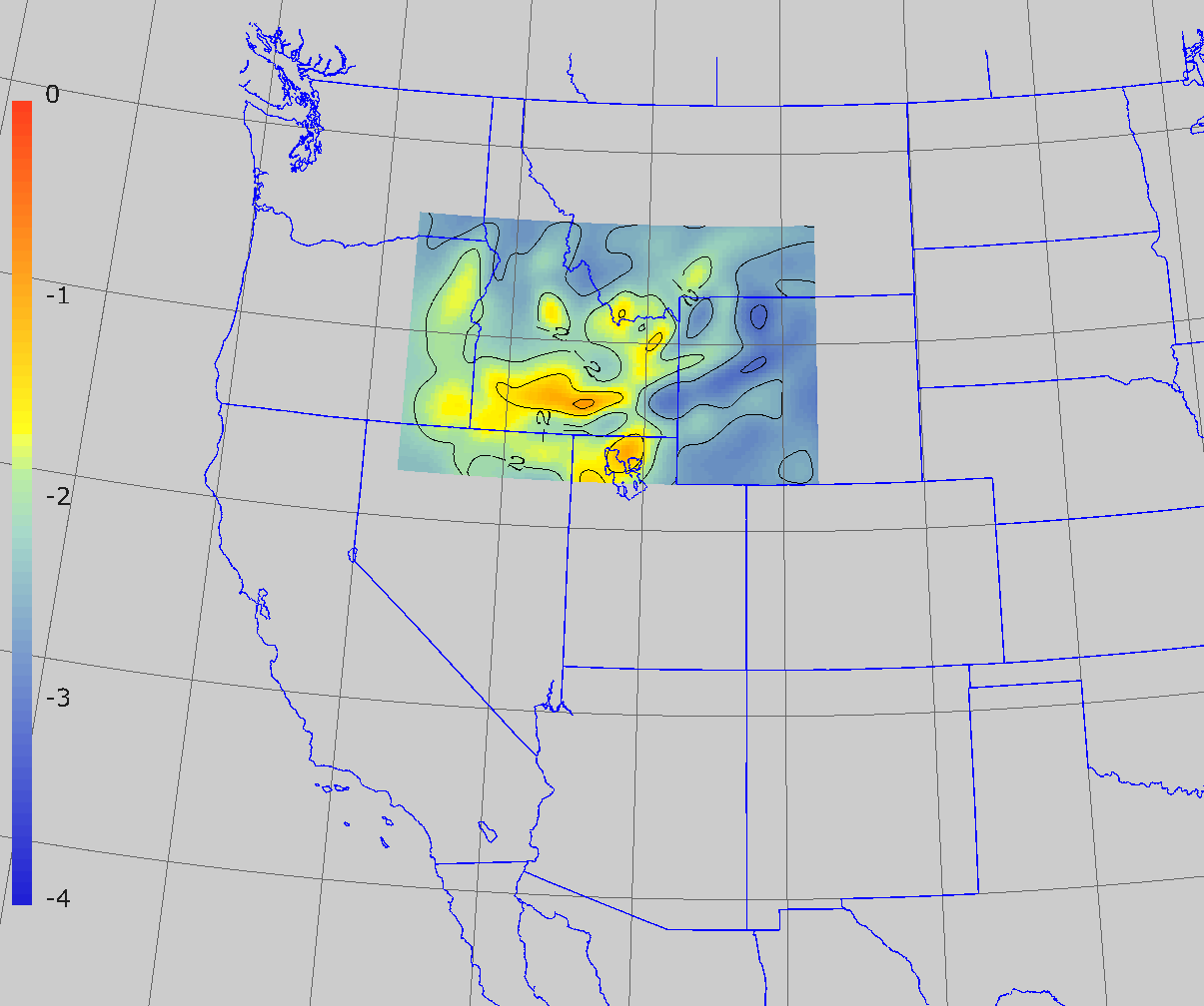
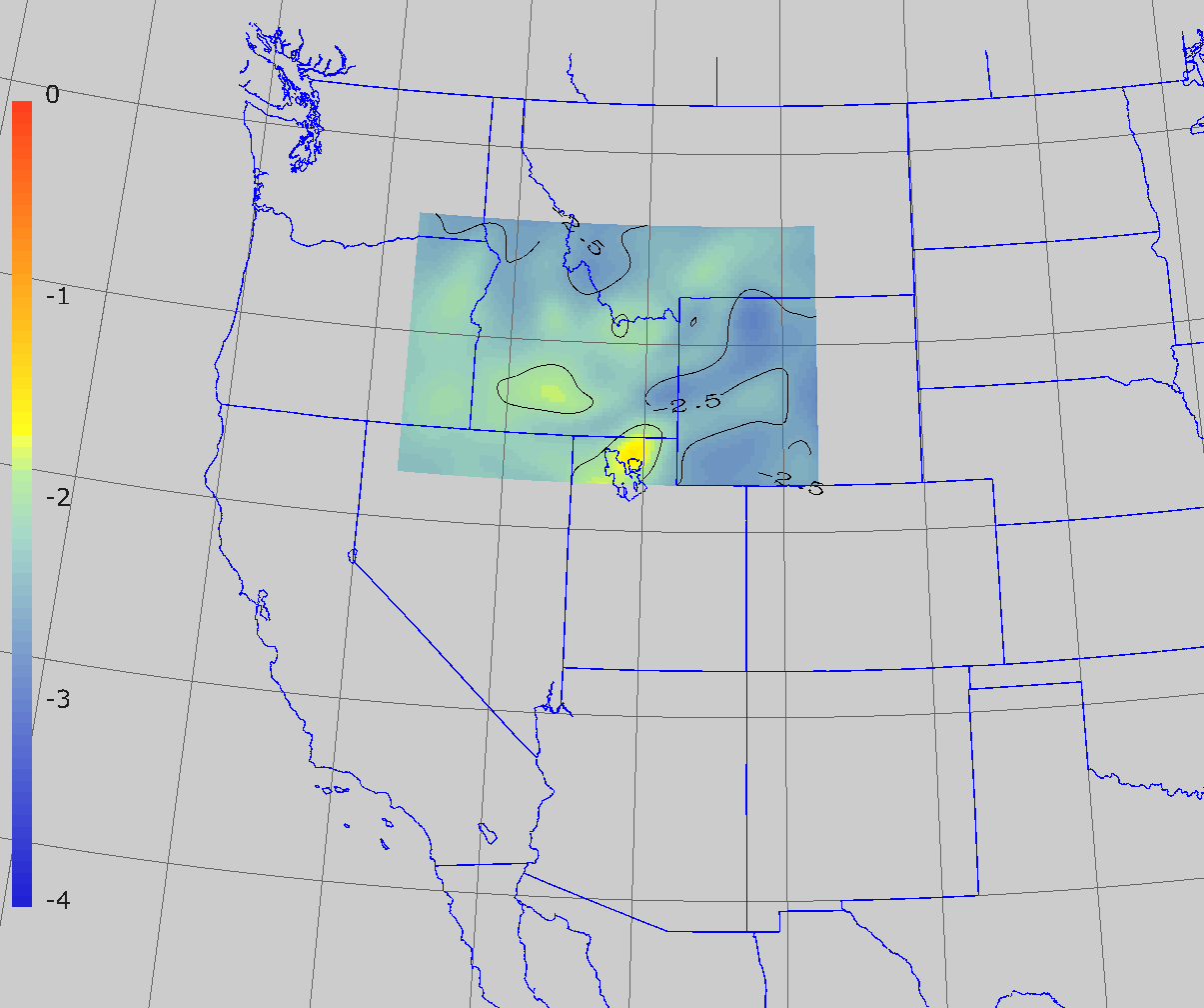
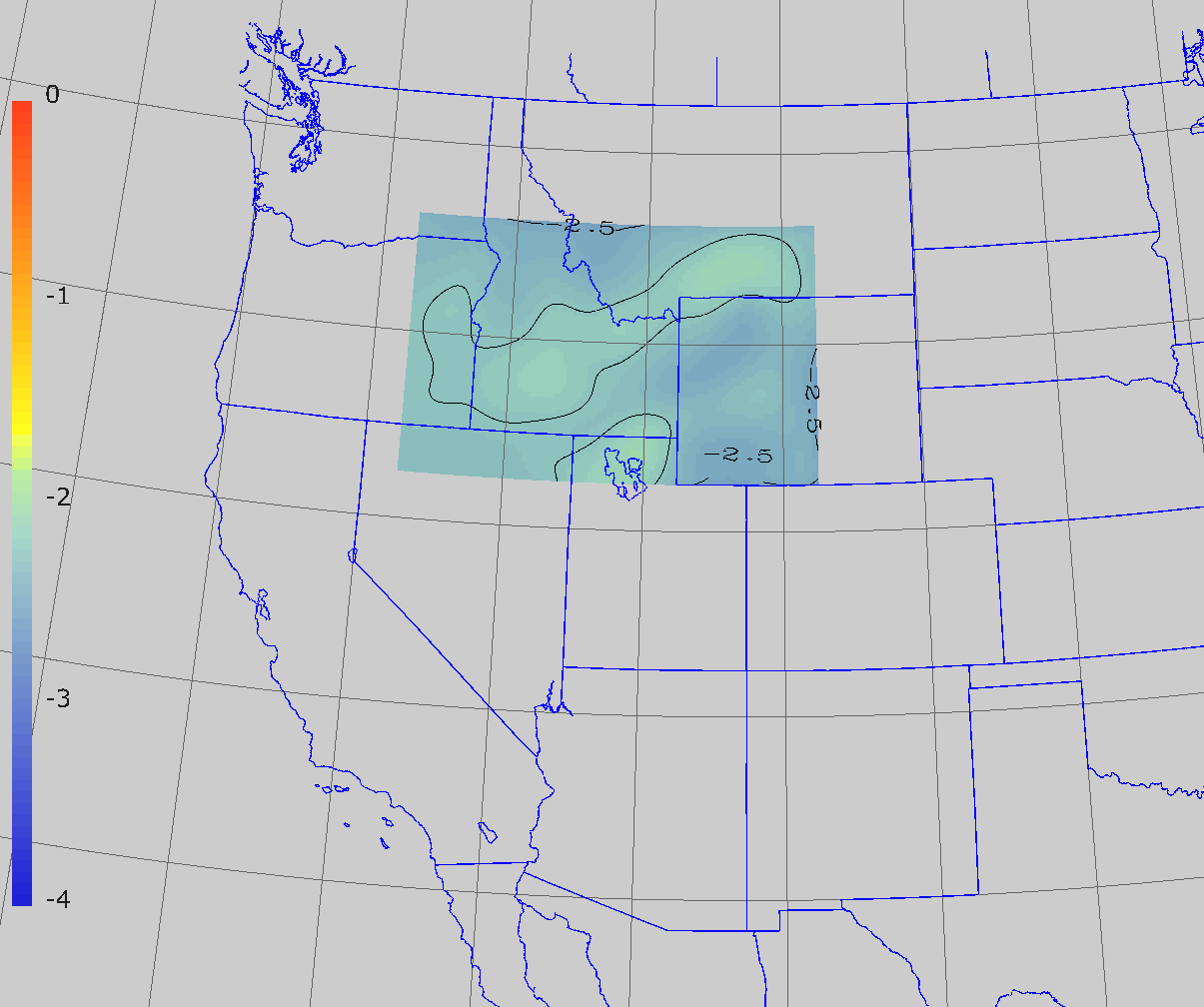
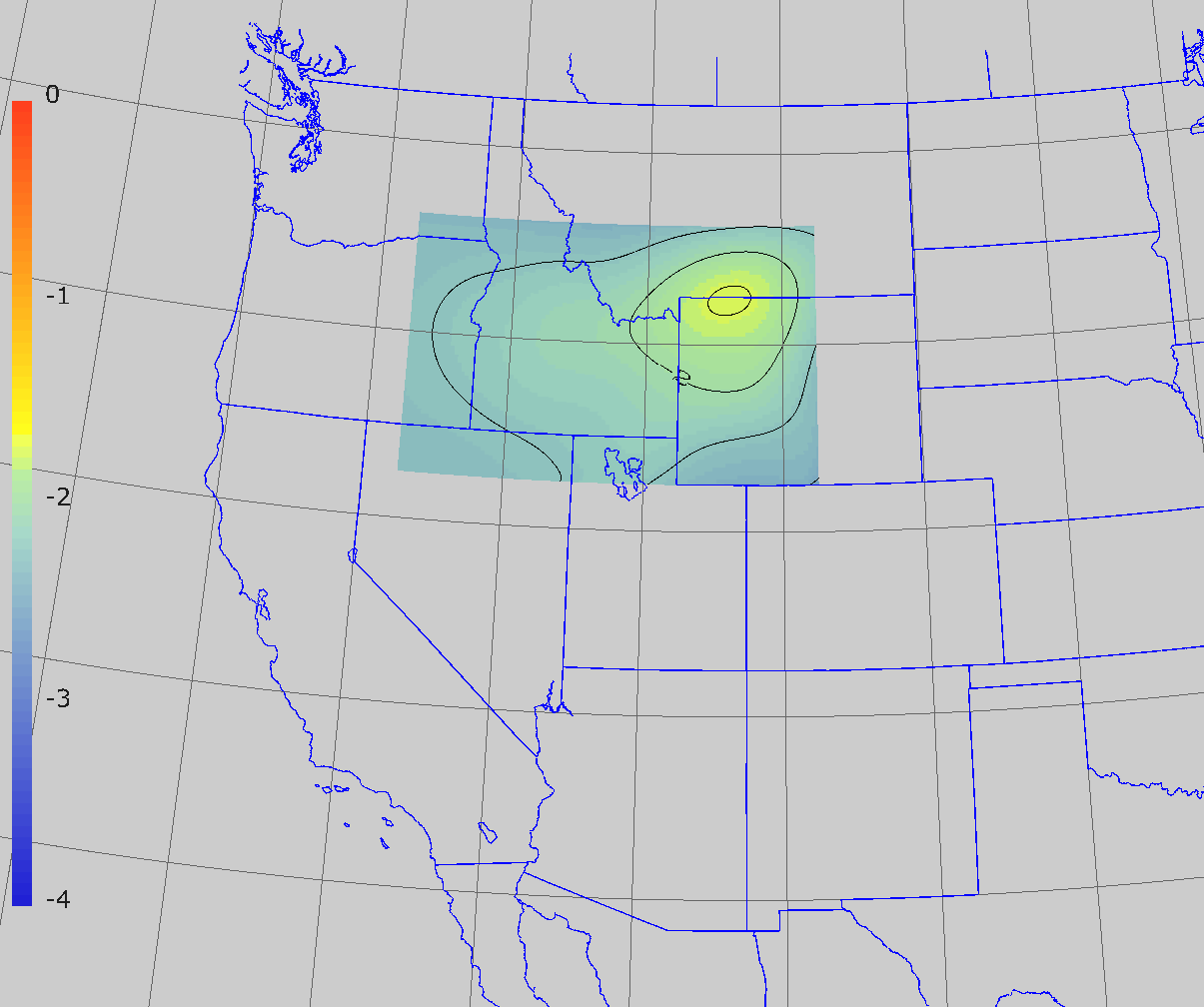
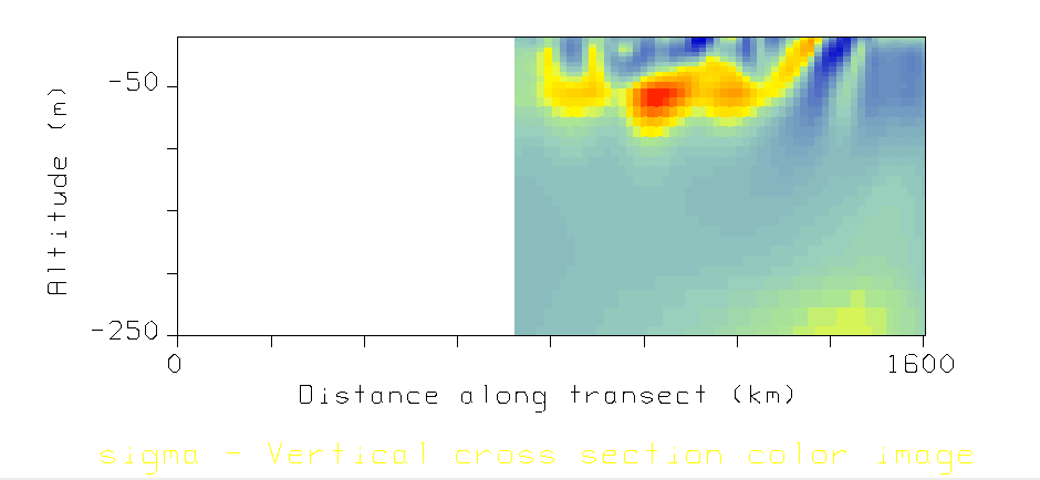
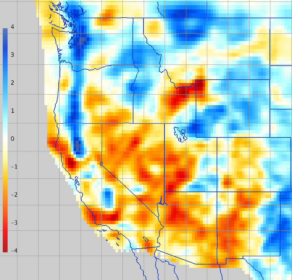
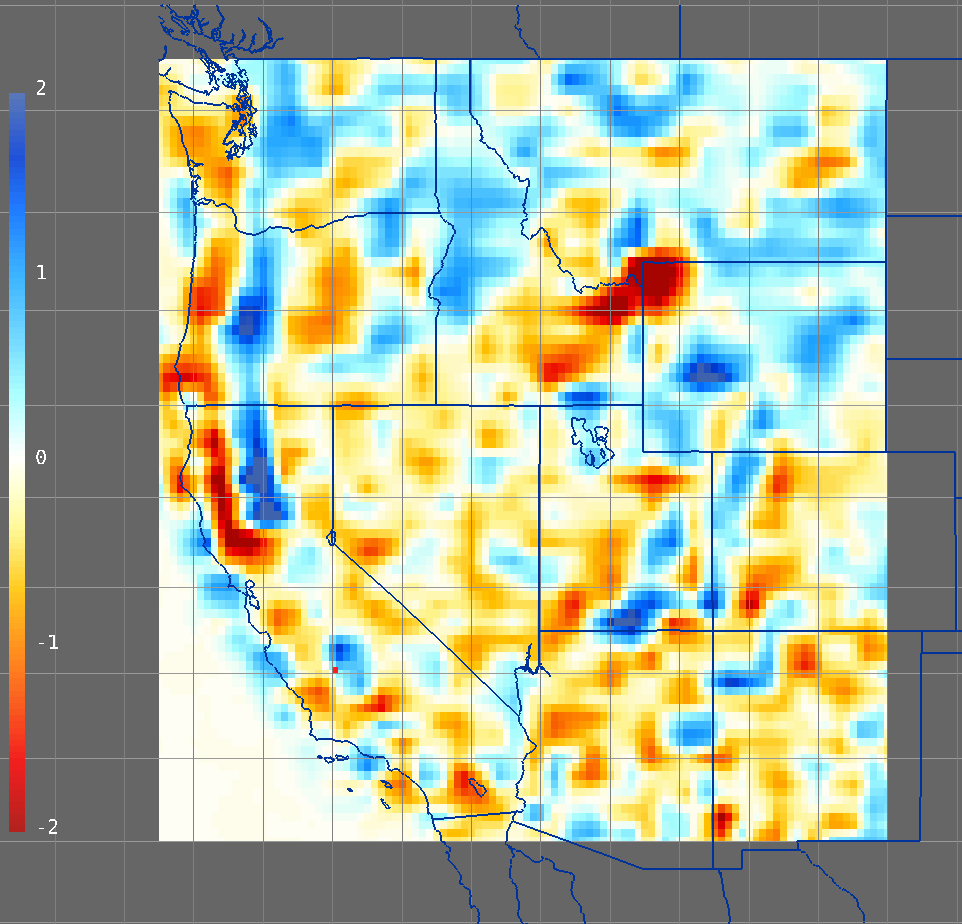
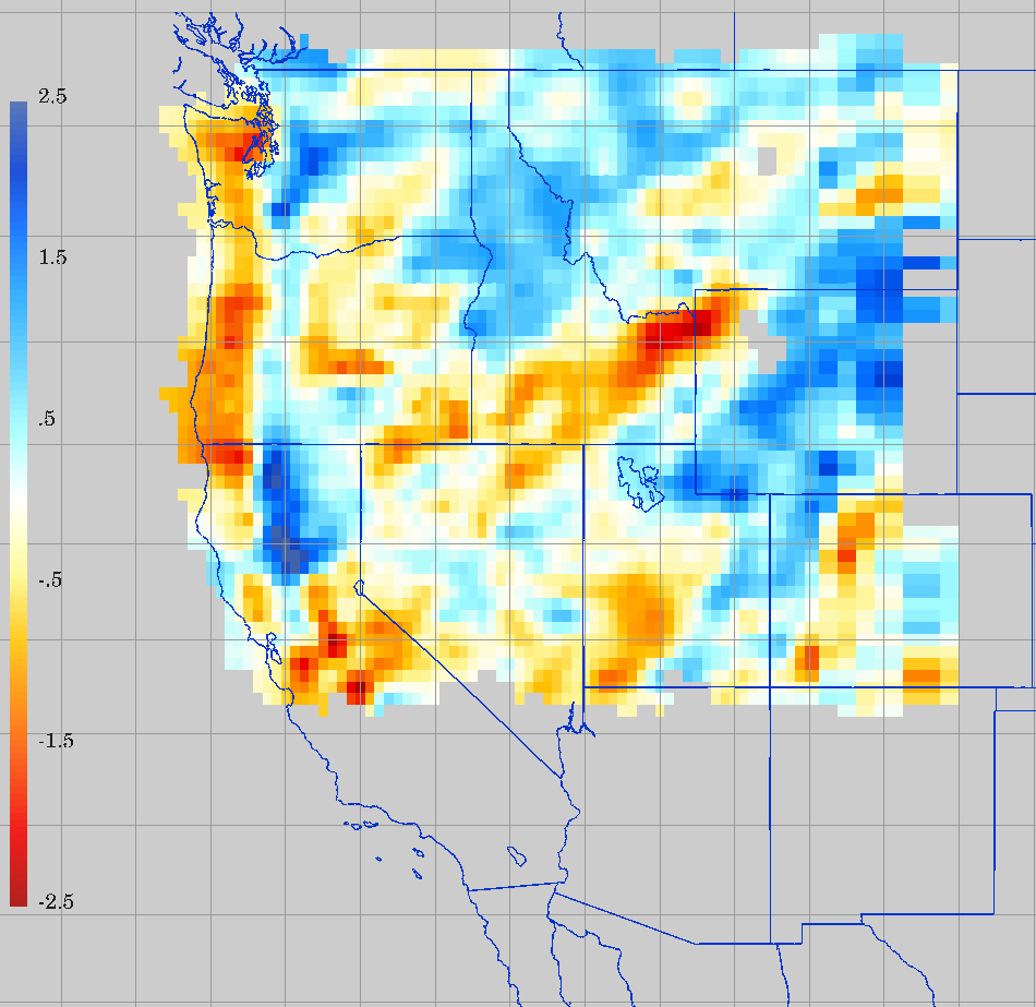
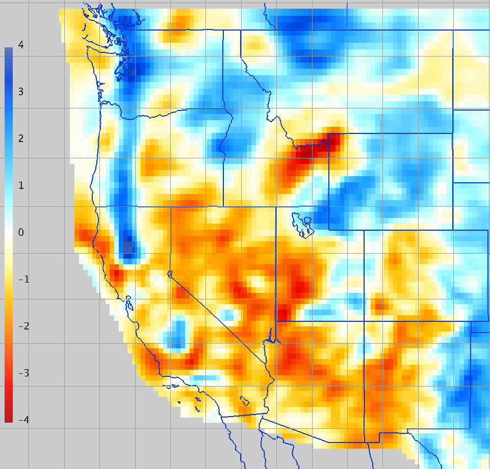
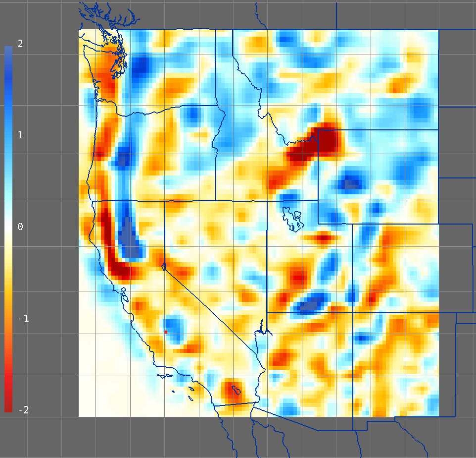
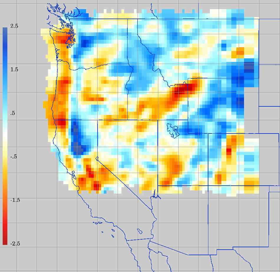
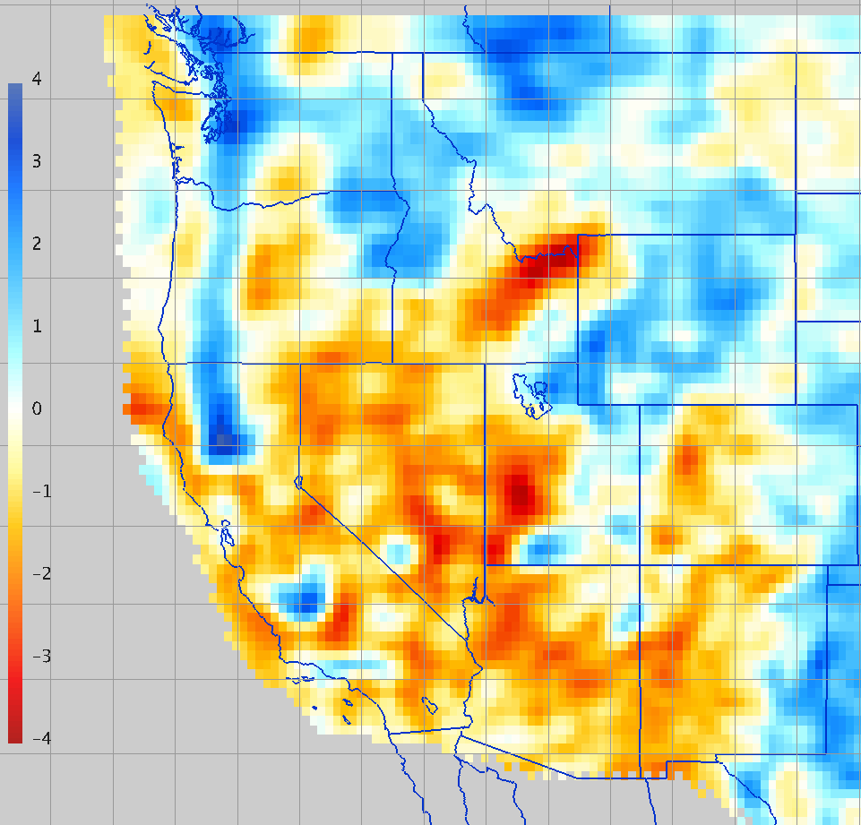
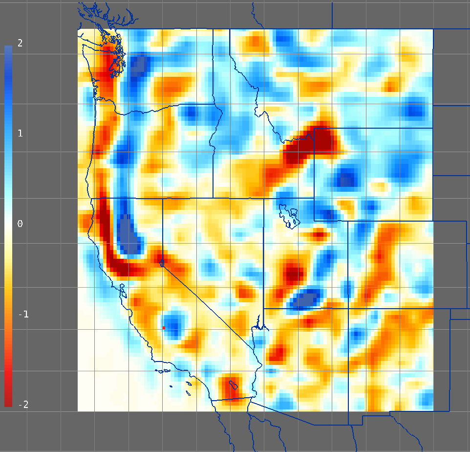
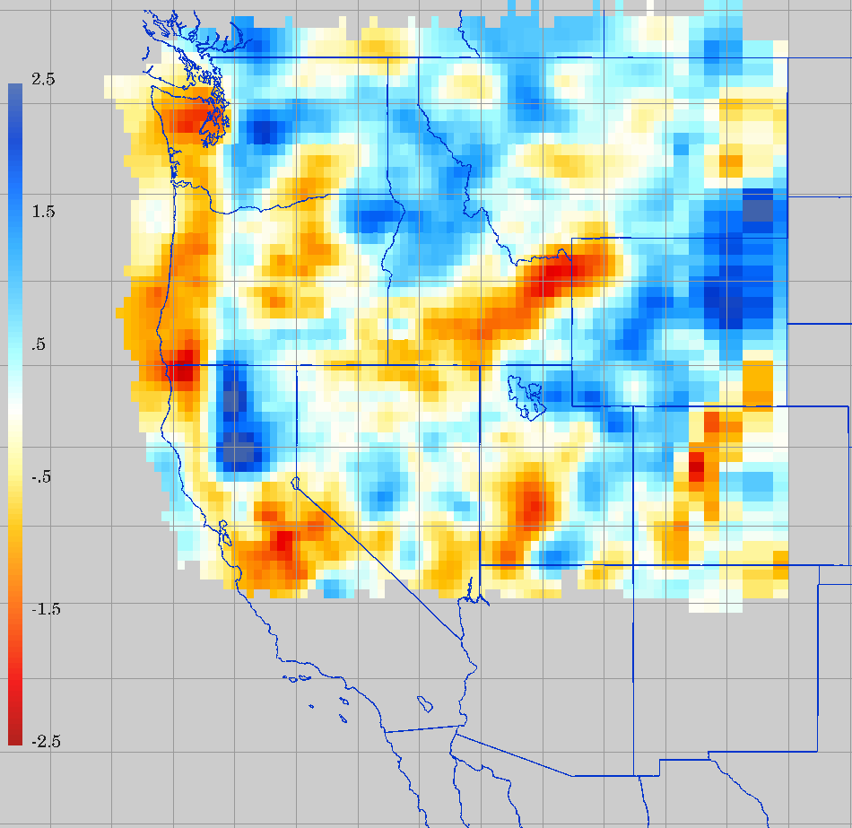
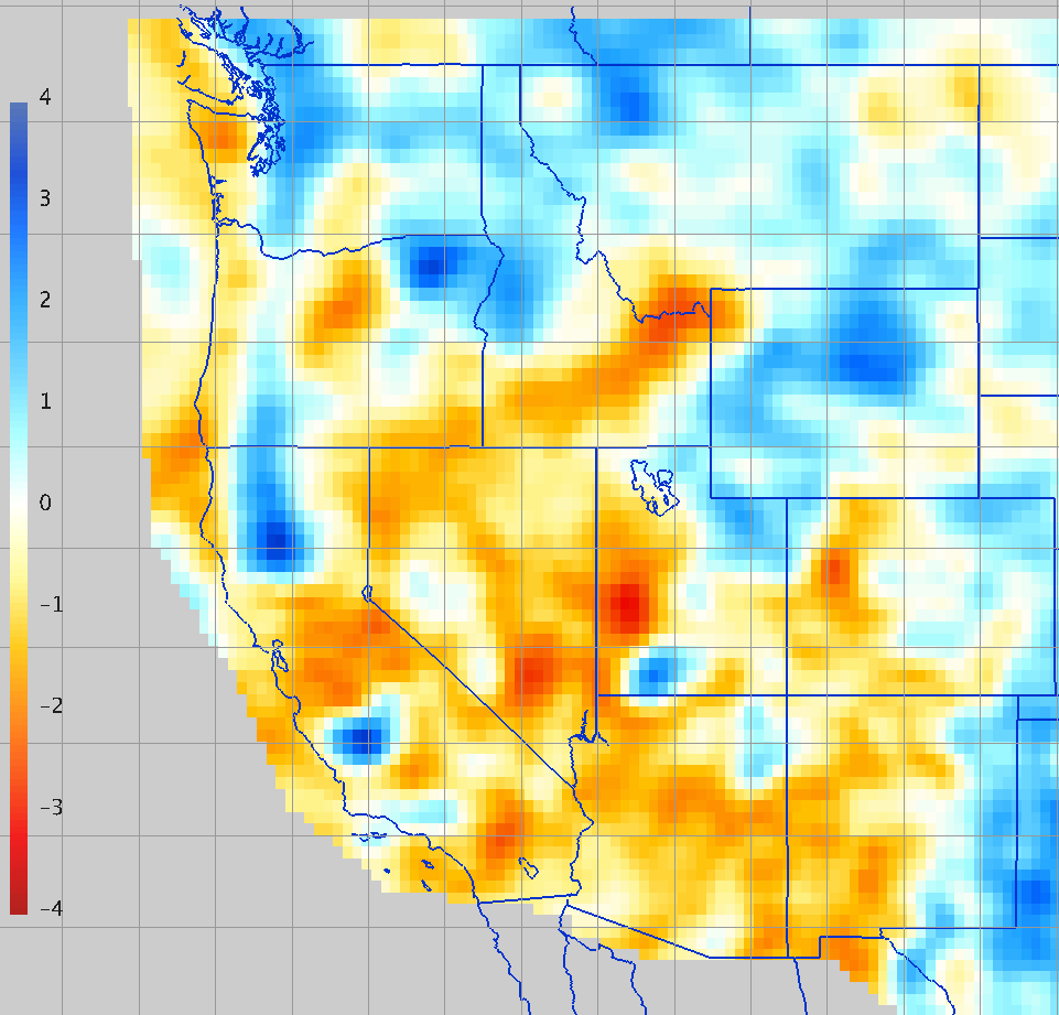
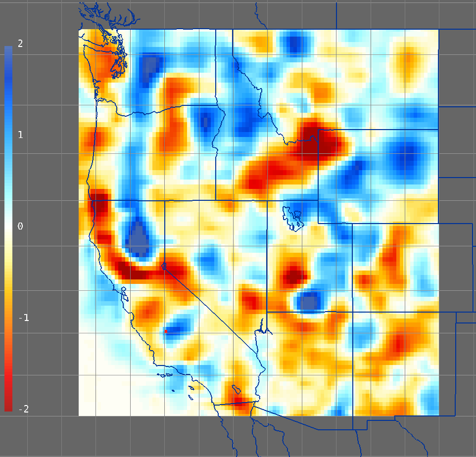
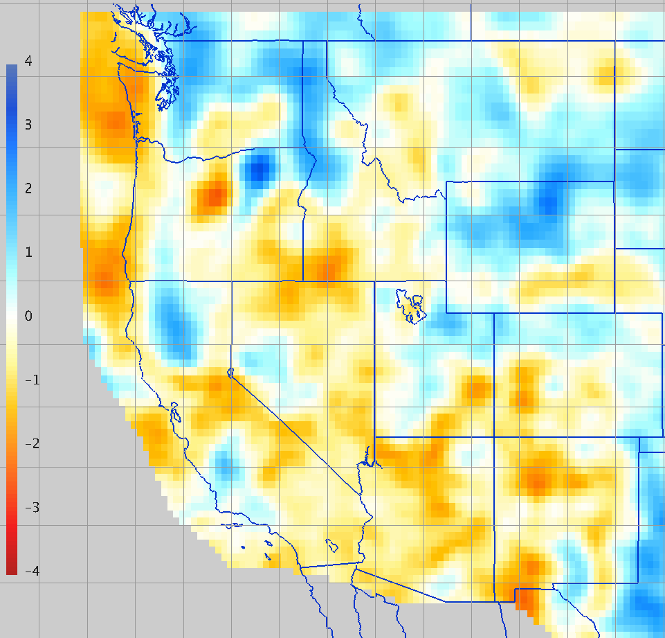
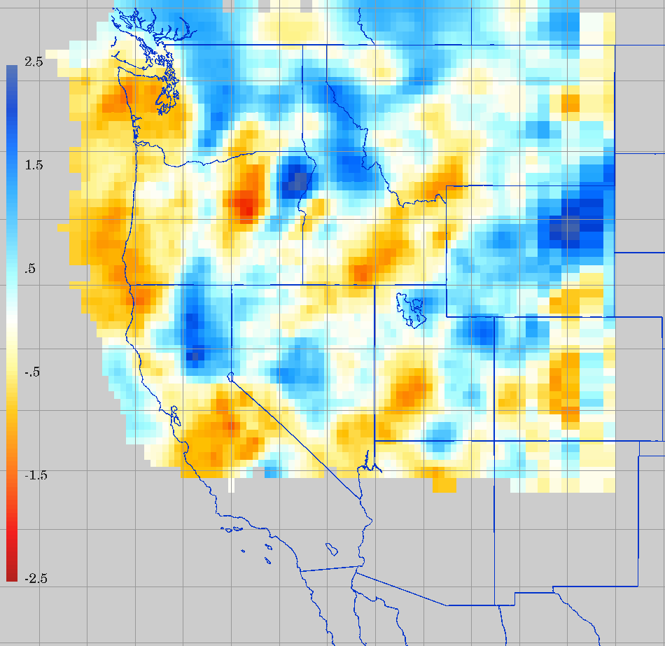
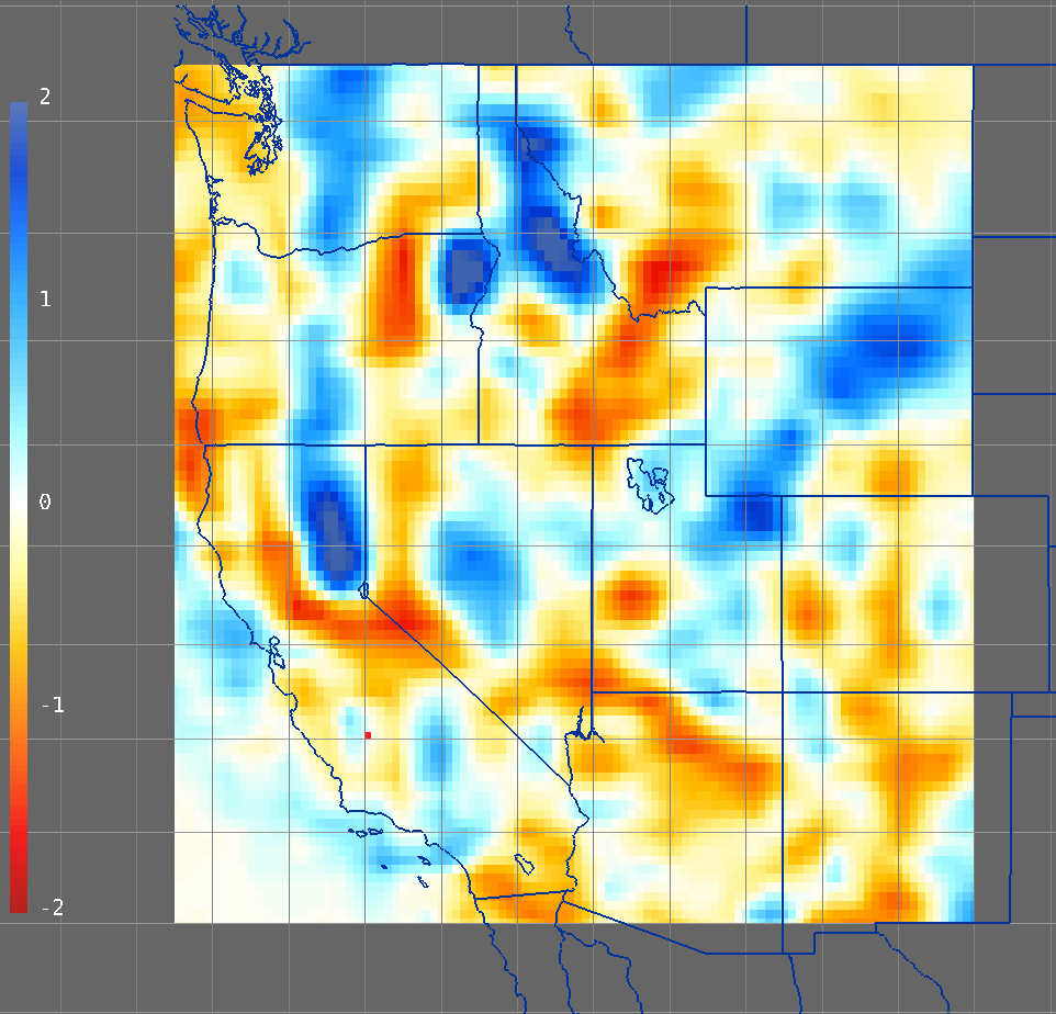
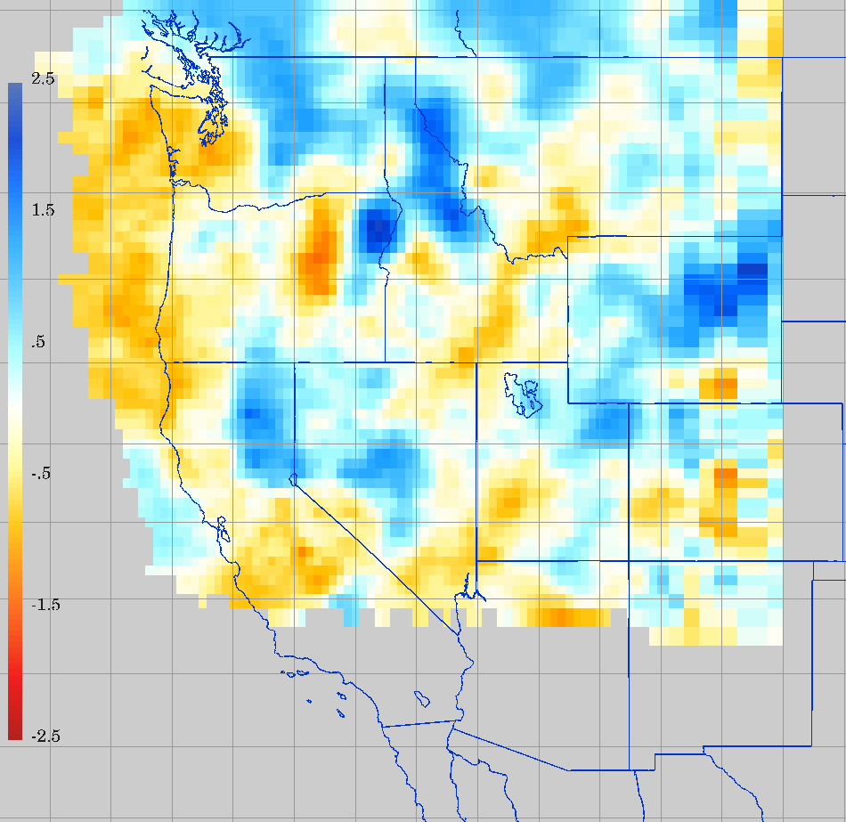
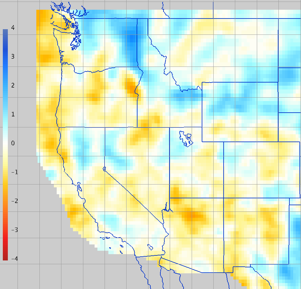
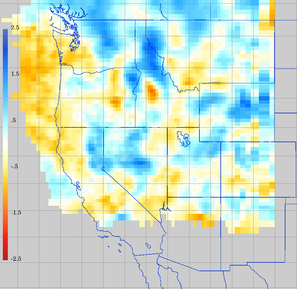
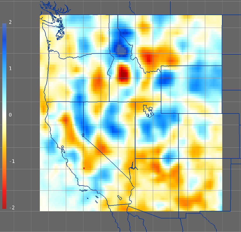
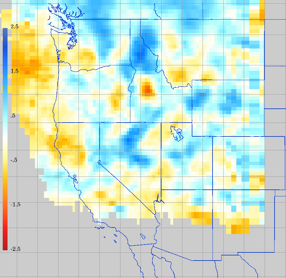
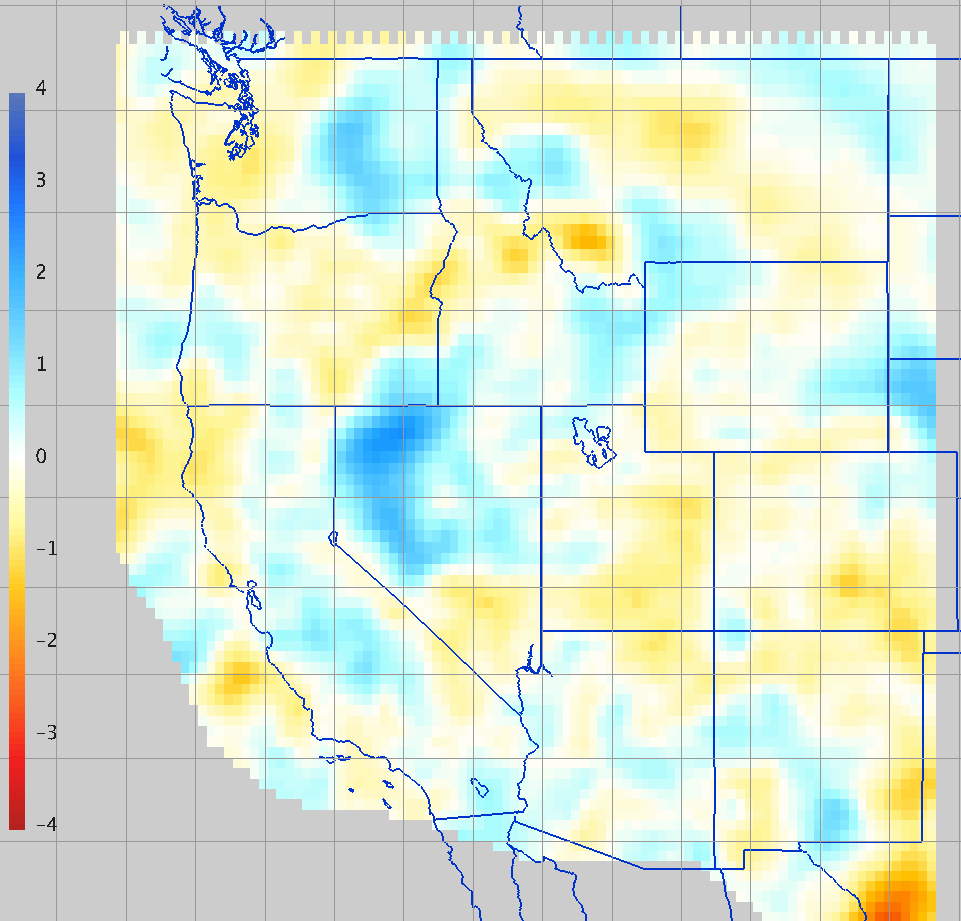
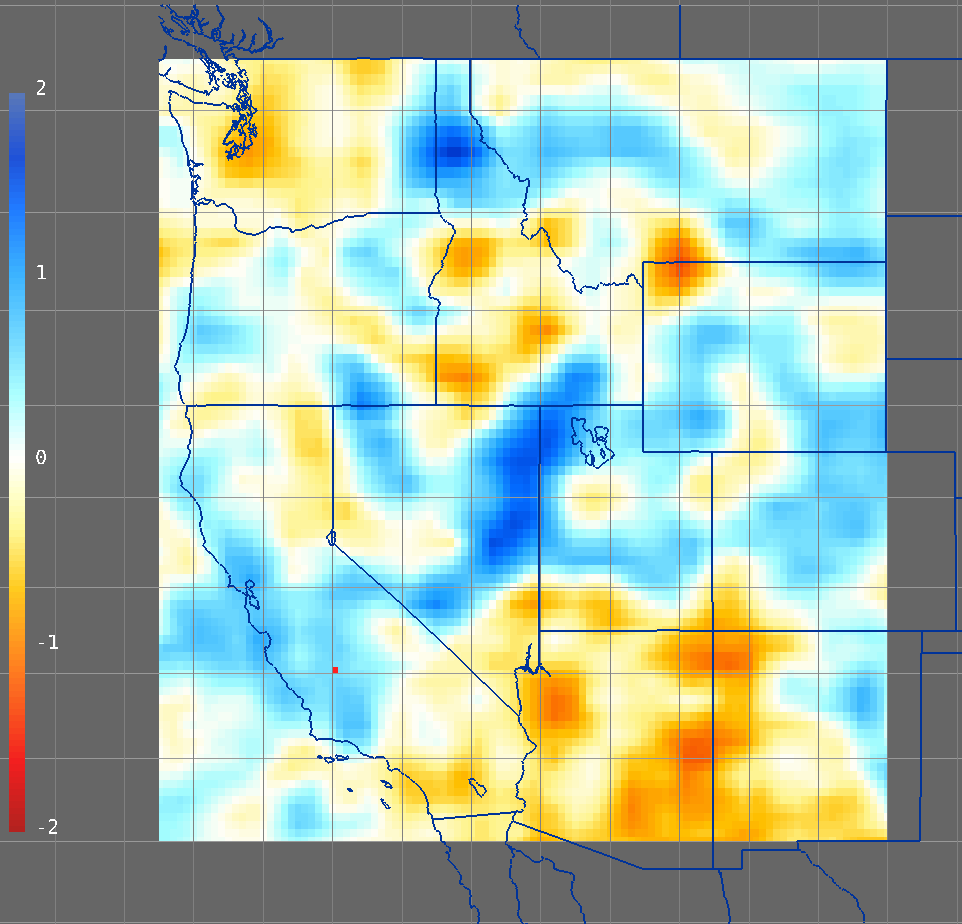
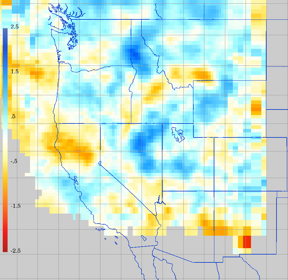
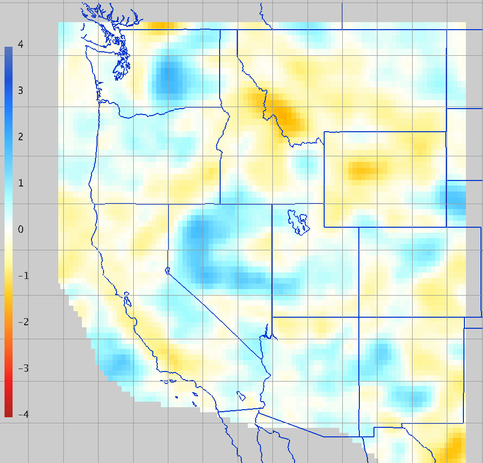
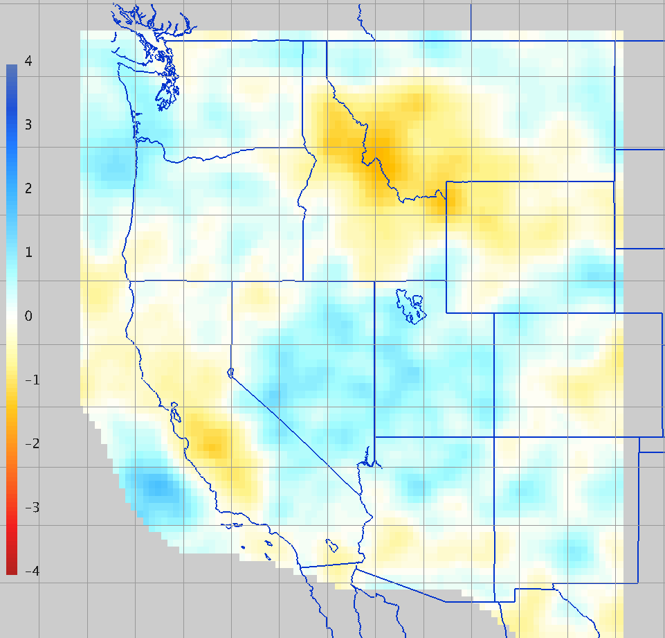
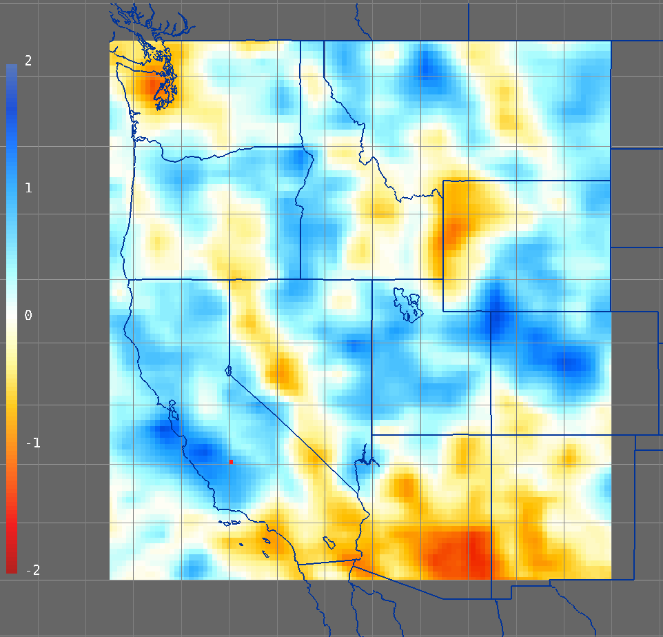
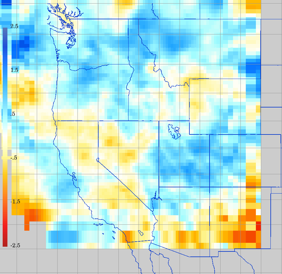
Comparing recent Western US Earth Structure Models
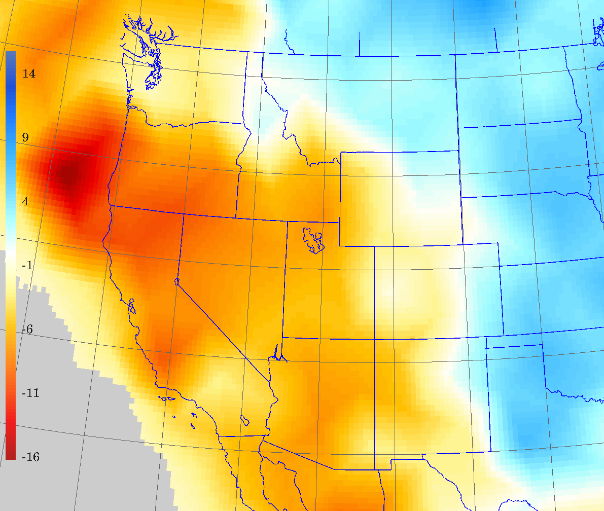
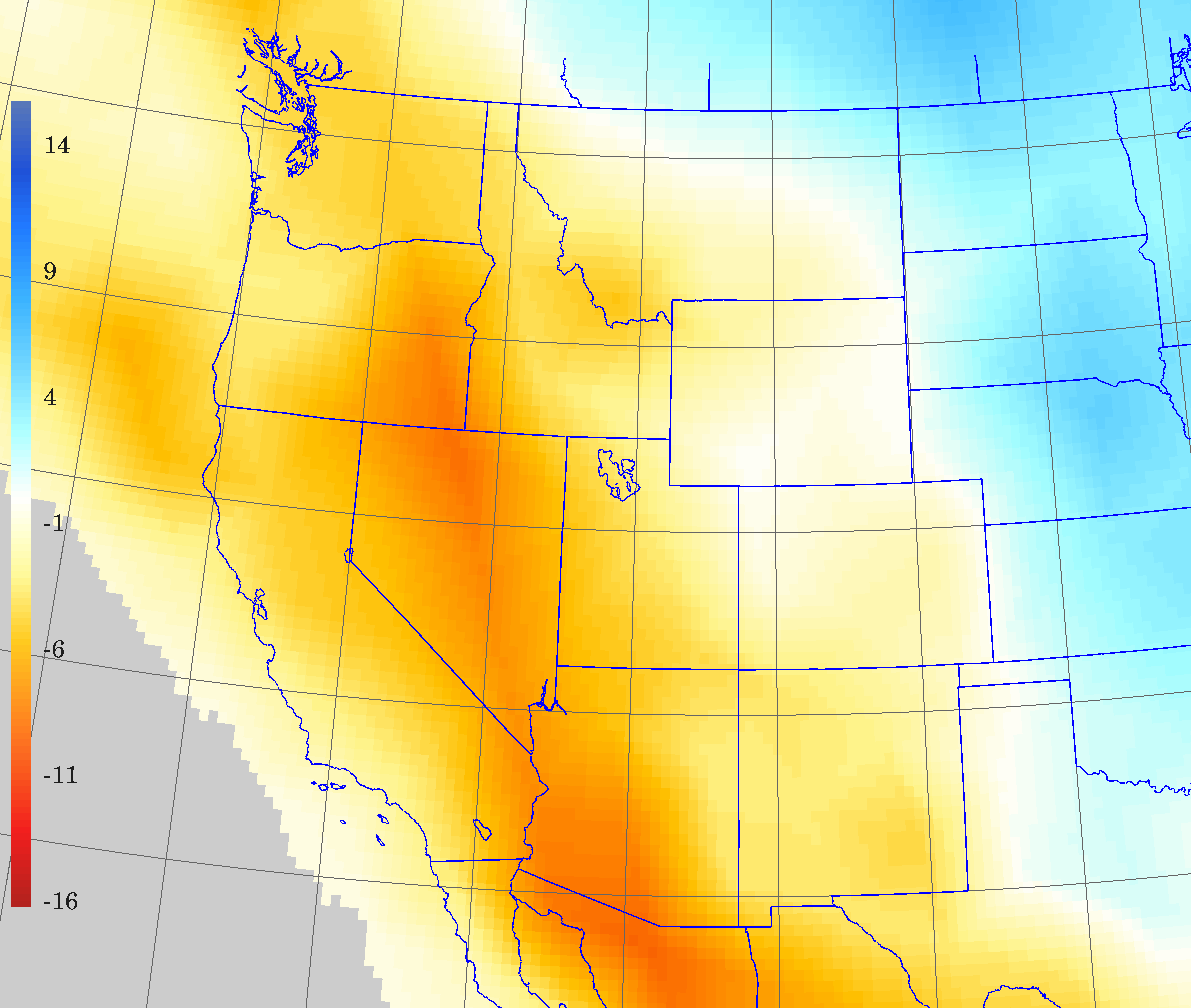
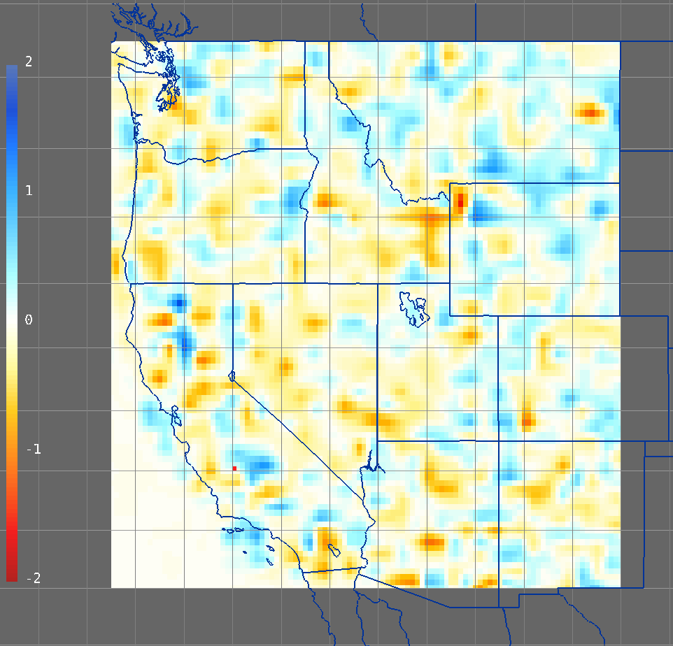
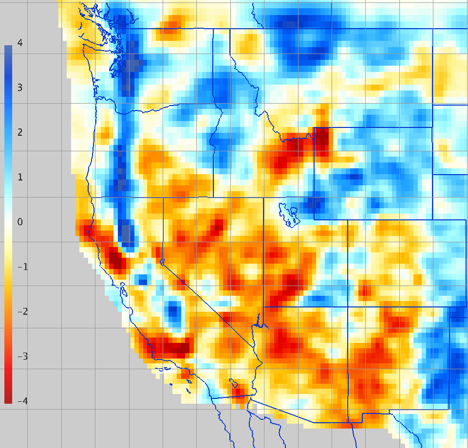
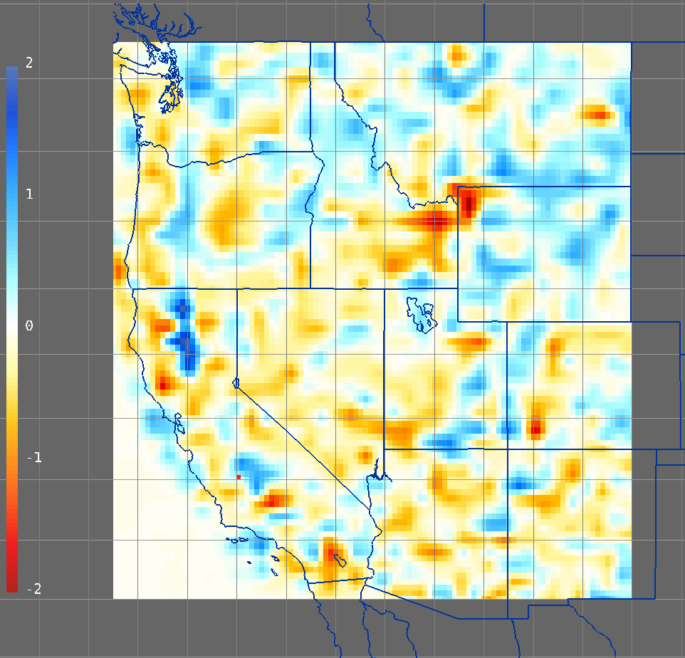
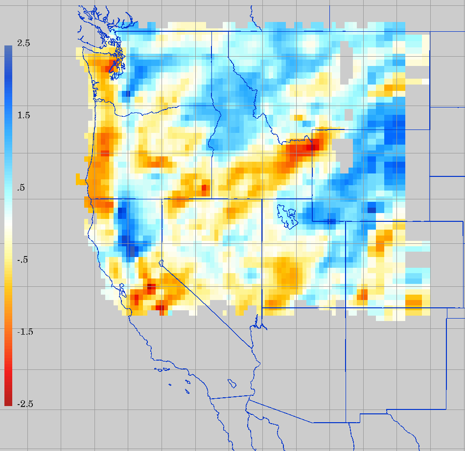
From recent 3D models of structure of the western U.S., available online, here is a comparison using images made from IDV interactive displays. There are horizontal cross-sections at five depths, and a vertical cross section (the cross section position line is shown in the NWUS model map displays). Color legends have been adjusted to approximately the same range of colors in each level. White is zero anomaly in all displays.
All maps have the same projection and area. The IDV interpolated some model grids to get values at the levels shown here, in the cases where the model did not provide data at these levels.
To compare two displays, open one image in a new tab, and go to the this page again and open the second image in another new tab. Then use your browser tabs to do a "blink comparison," switching between them.
S Velocity Anomalies
Model name Depths: 50 km 75 km 100 km 150 km 250 km vertical
X sectionNWUS11 S 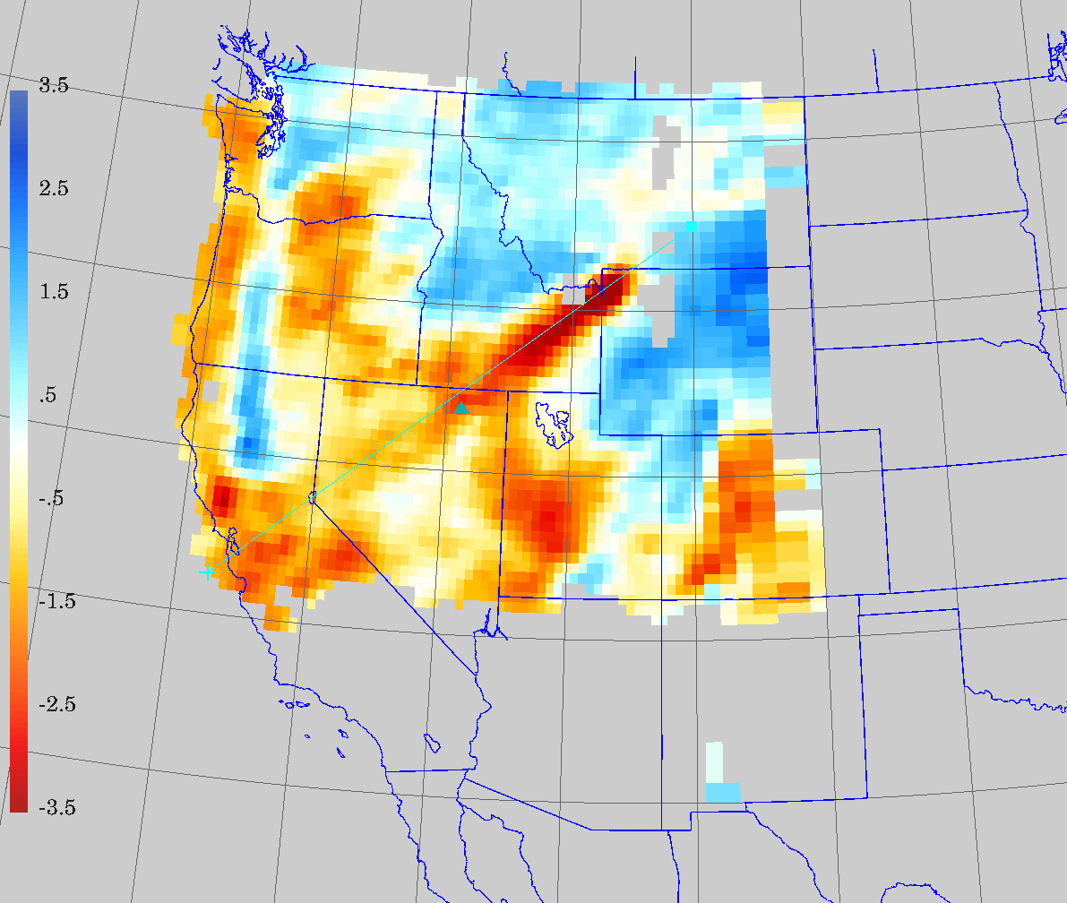
DNA10-S 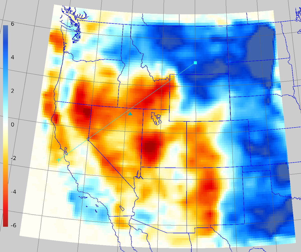
UO_wUS_6_10_dVs 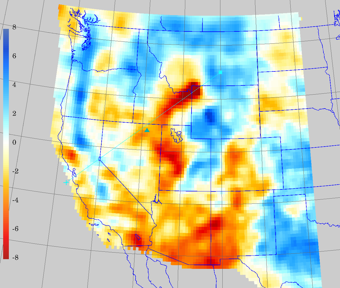
NA07 dVs 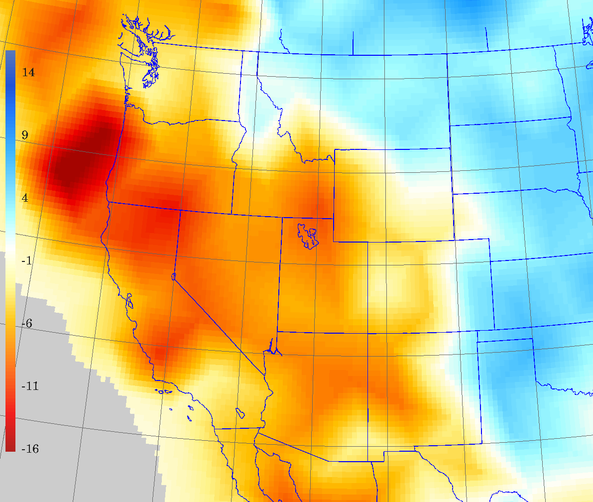
PNW 10-S 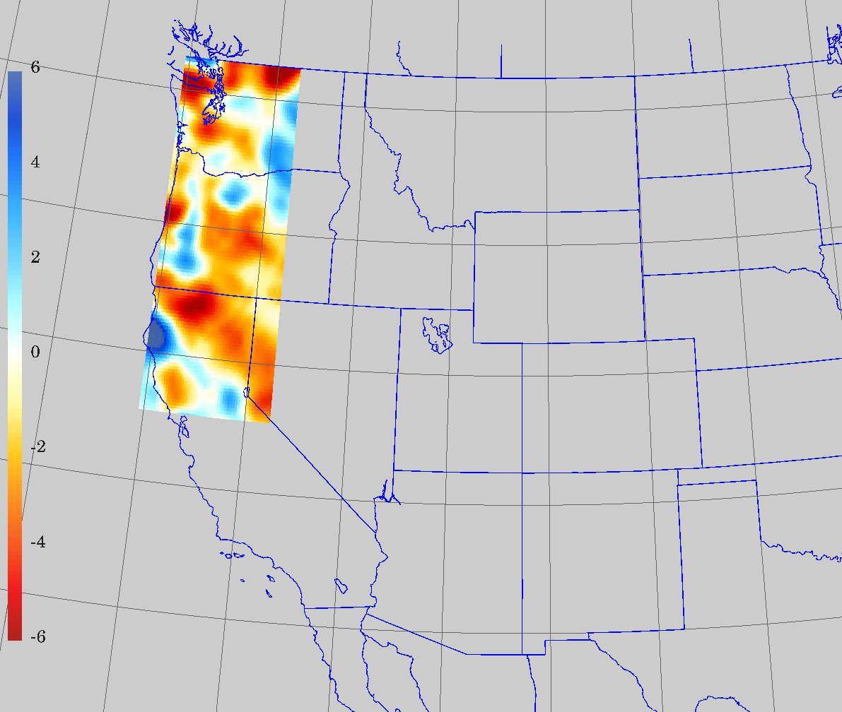
SPRY
Magnetotelluric model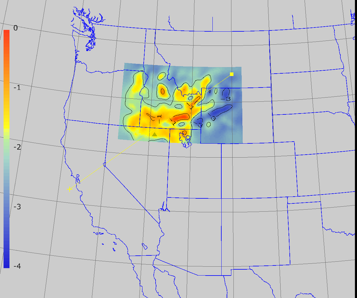
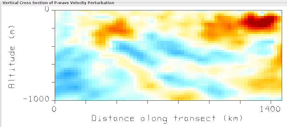
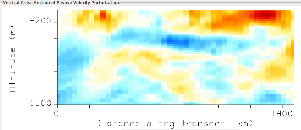
P Velocity anomalies
Depths Models: MITP, January 2010 UO_wUS_6_10_dVp DNA09 NWUS11-P Vertical cross-section 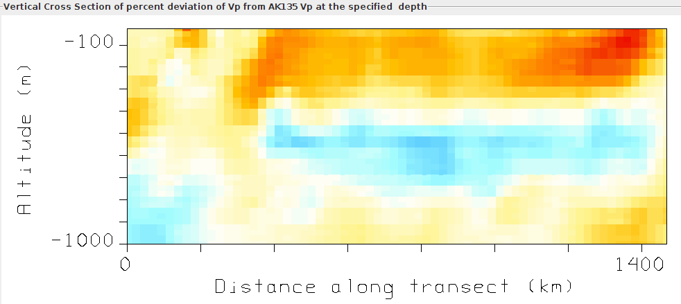
25 km 
60 km 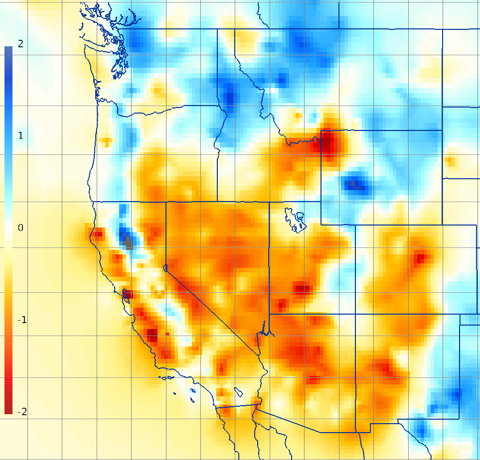
75 km 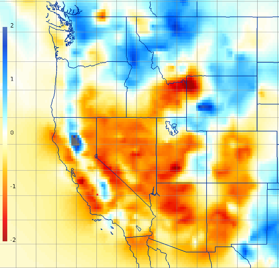
100 km 
125 km 

150 km 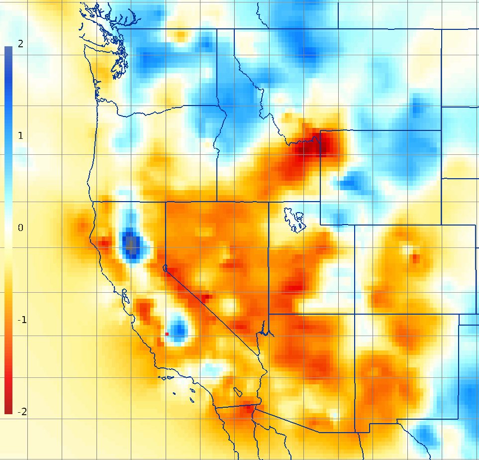
175 km 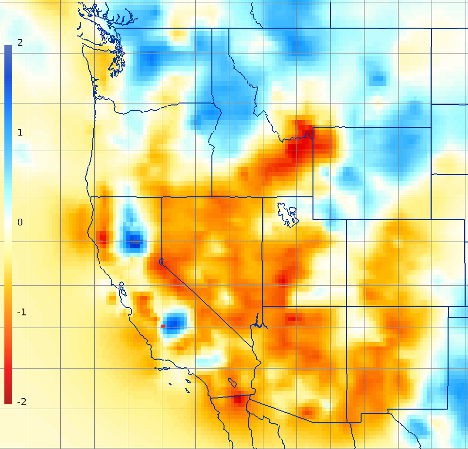
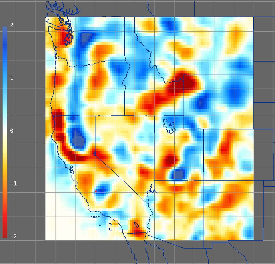
200 km 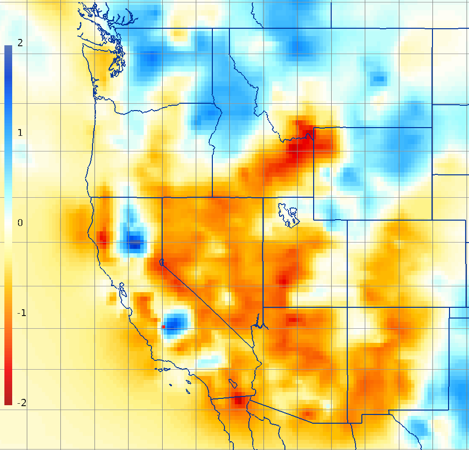
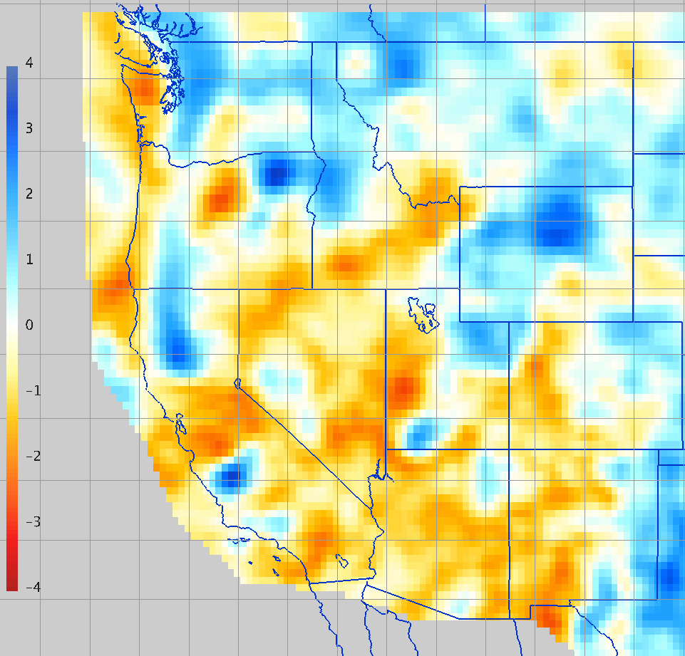
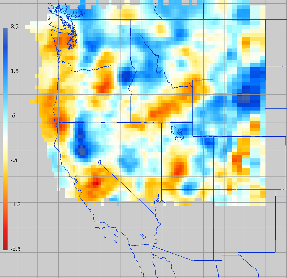
267 km 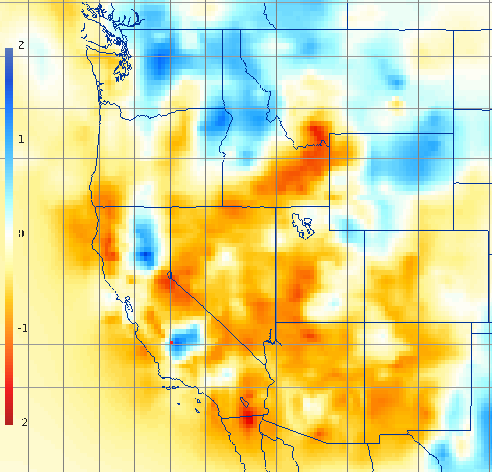
300 km 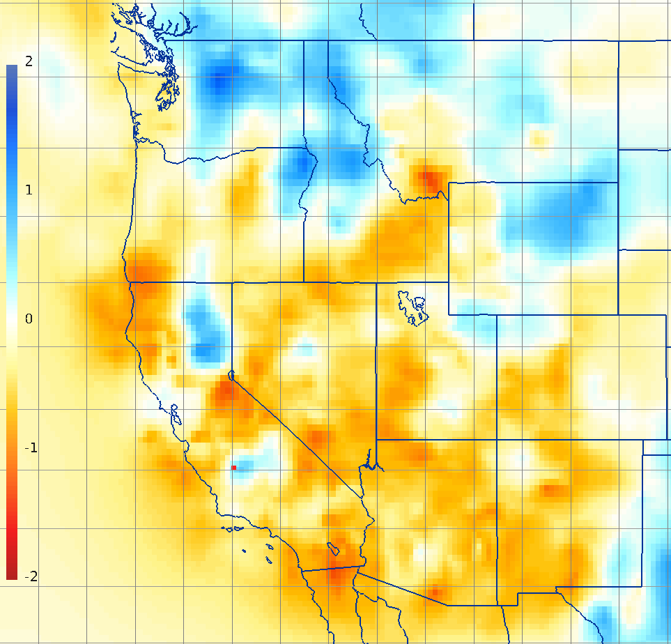
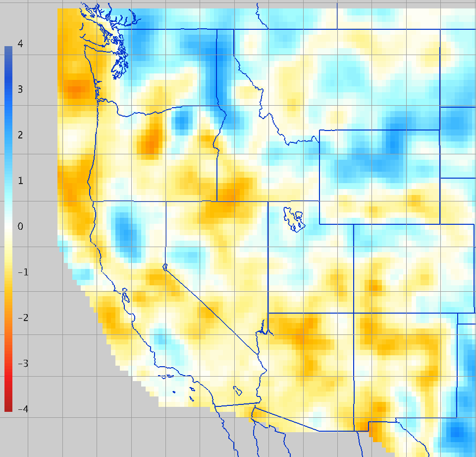
350 km 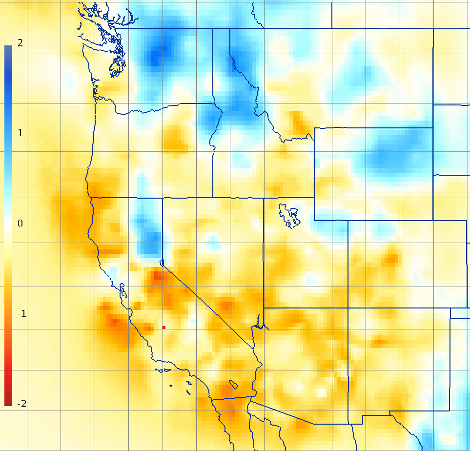
400 km 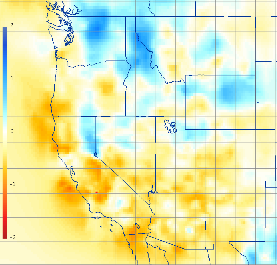
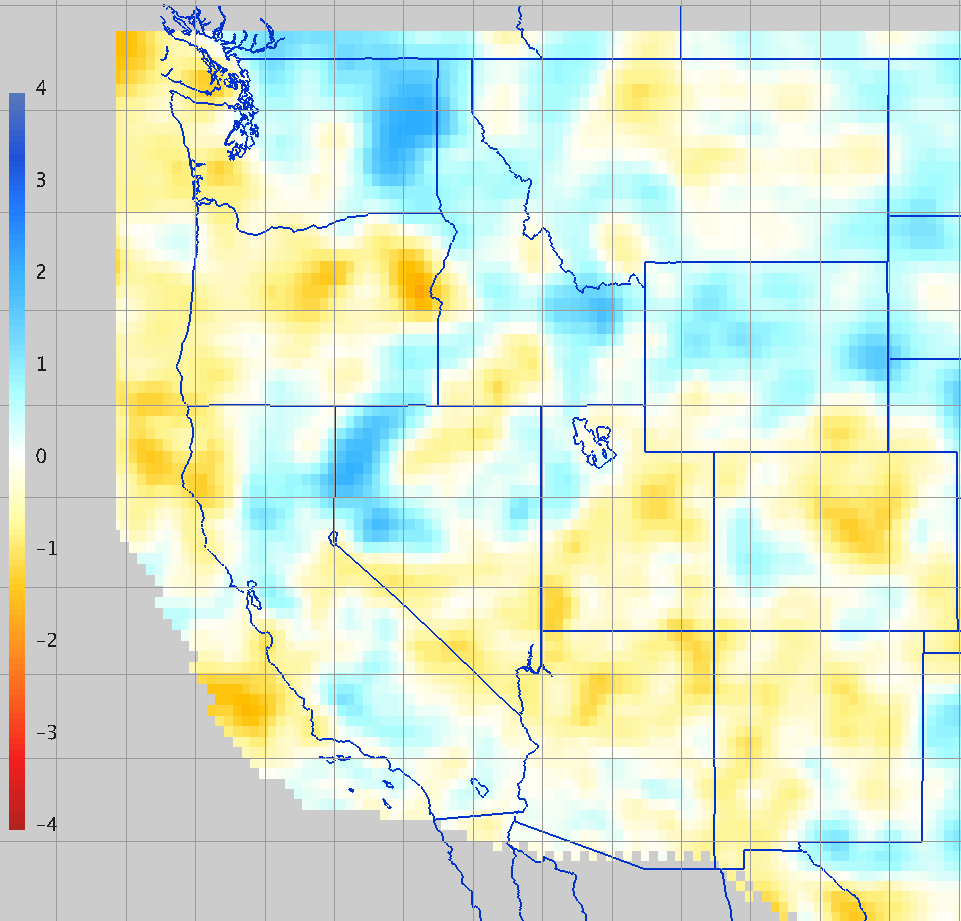
450 km 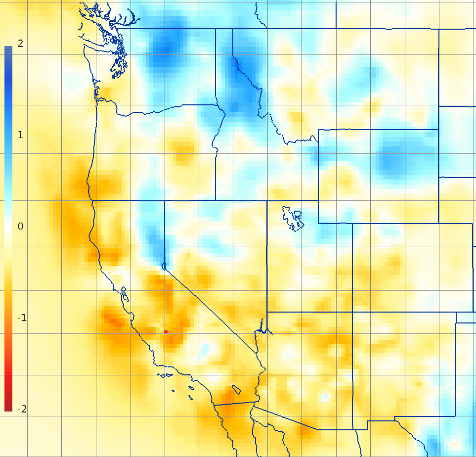
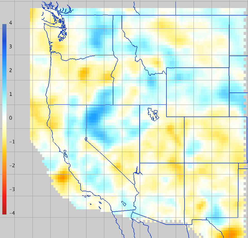

500 km 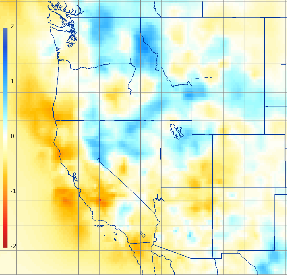
600 km 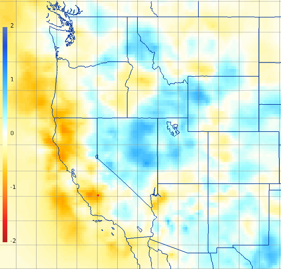
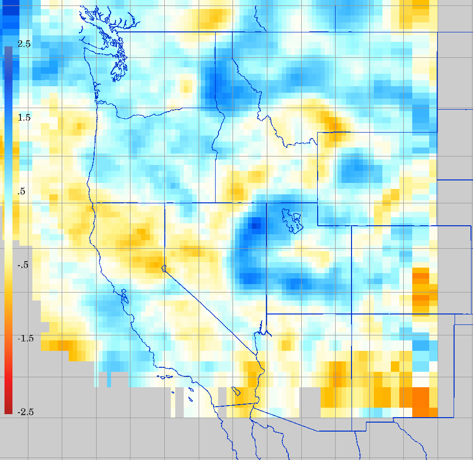
700 km 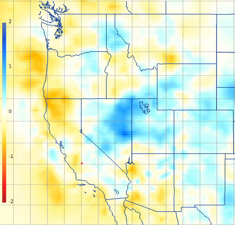
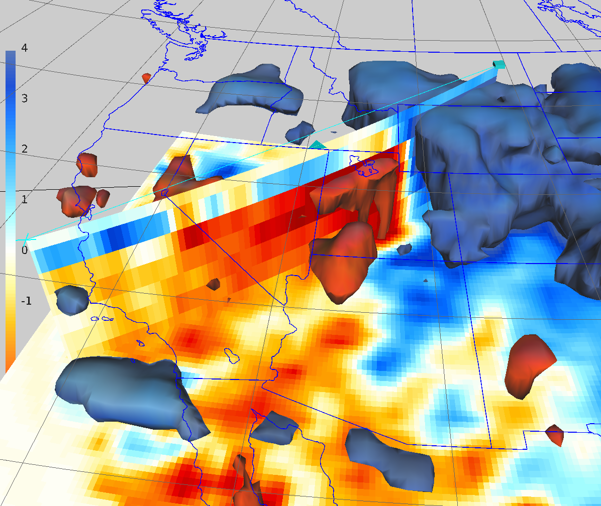
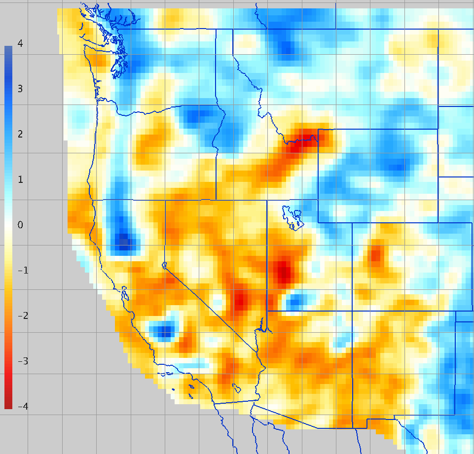
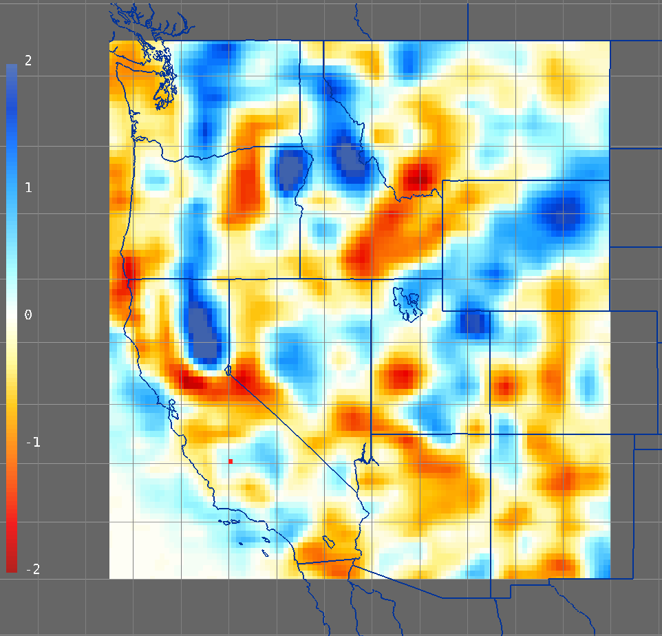
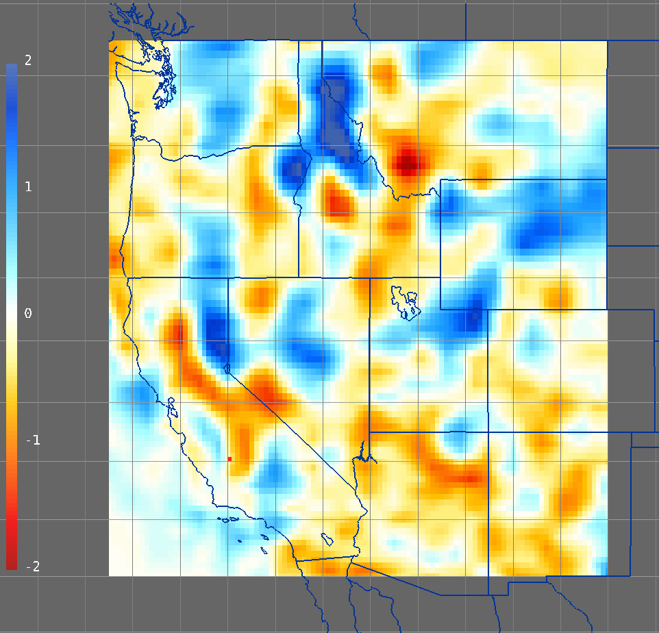
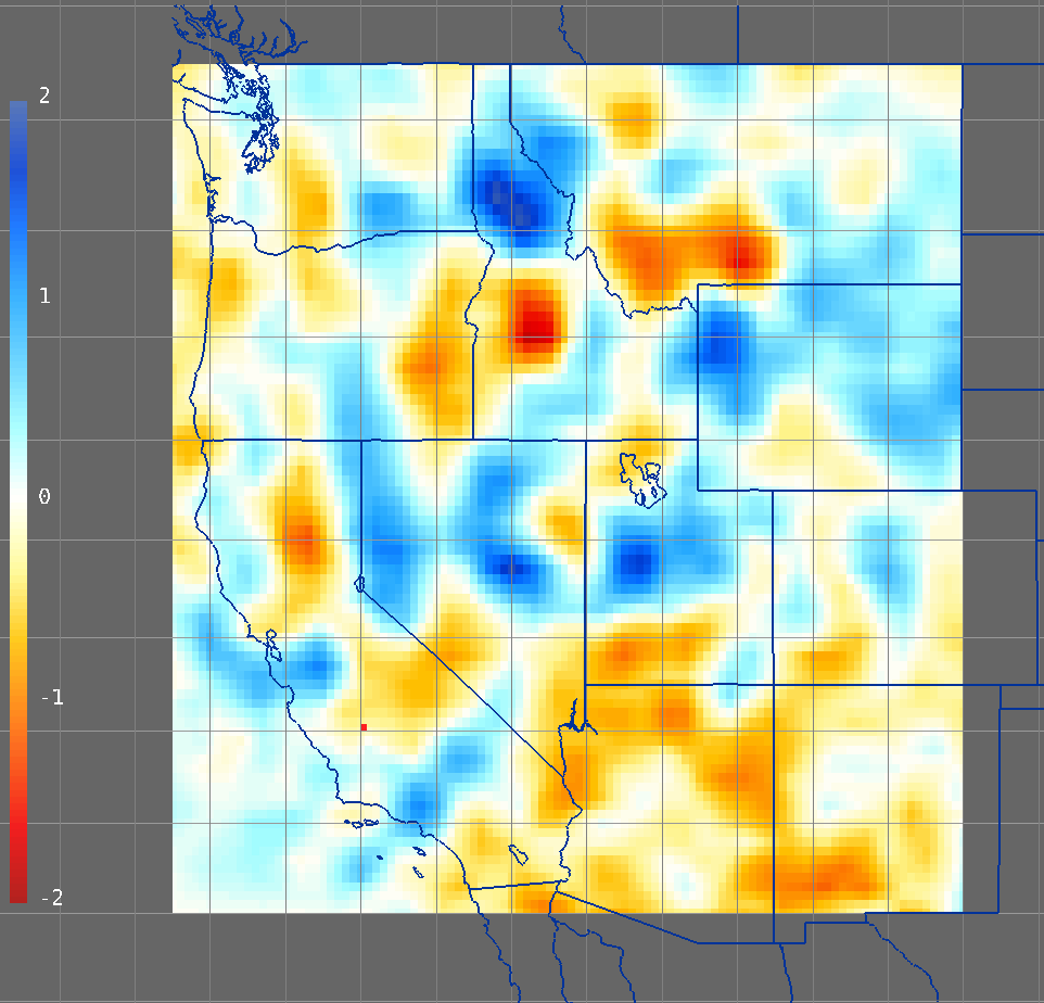
Use the IDV to Compare Different Models
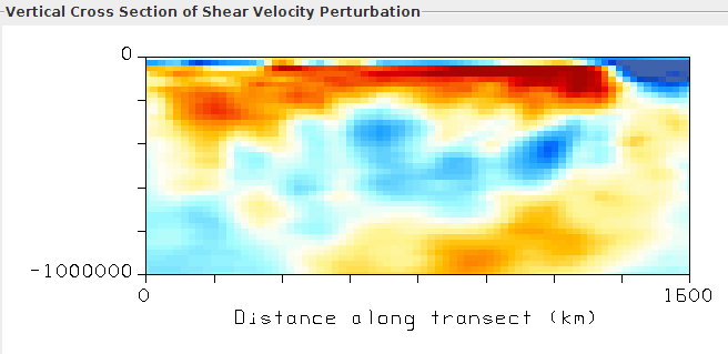
The IDV can do computations with 3D grids, including such things as differences between two models or between a model and a reference data set.
The difference between two seismic tomography models can be computed and displayed by using the IDV's computational ability ("formulas"). IDV automatically does interpolations and unit conversions before making the display, such as if the two 3D grid cells' sizes or centers differ.
Isosurface and vertical cross section of difference of